Object Recognition with Convolutional Neural Networks in the Keras Deep Learning Library

Download your PDF containing all 14 lessons.

Get your daily lesson via email with tips and tricks.

Loading The CIFAR-10 Dataset in Keras

The CIFAR-10 dataset can easily be loaded in Keras.

Keras has the facility to automatically download standard datasets like CIFAR-10 and store them in the ~/.keras/datasets directory using the cifar10.load_data() function. This dataset is large at 163 megabytes, so it may take a few minutes to download.

Once downloaded, subsequent calls to the function will load the dataset ready for use.

The dataset is stored as pickled training and test sets, ready for use in Keras. Each image is represented as a three dimensional matrix, with dimensions for red, green, blue, width and height. We can plot images directly using matplotlib.

# Plot ad hoc CIFAR10 instances
from keras.datasets import cifar10
from matplotlib import pyplot
from scipy.misc import toimage
# load data
(X_train, y_train), (X_test, y_test) = cifar10.load_data()
# create a grid of 3x3 images
for i in range(0, 9):
	pyplot.subplot(330 + 1 + i)
	pyplot.imshow(toimage(X_train[i]))
# show the plot
pyplot.show()

Running the code create a 3×3 plot of photographs. The images have been scaled up from their small 32×32 size, but you can clearly see trucks horses and cars. You can also see some distortion in some images that have been forced to the square aspect ratio.

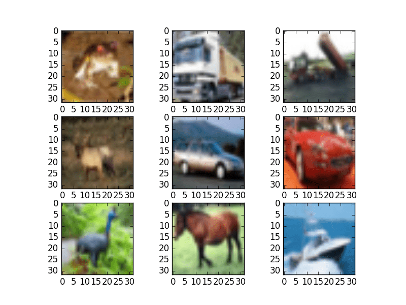
Small Sample of CIFAR-10 Images

Simple Convolutional Neural Network for CIFAR-10

The CIFAR-10 problem is best solved using a Convolutional Neural Network (CNN).

We can quickly start off by defining all of the classes and functions we will need in this example.

# Simple CNN model for CIFAR-10
import numpy
from keras.datasets import cifar10
from keras.models import Sequential
from keras.layers import Dense
from keras.layers import Dropout
from keras.layers import Flatten
from keras.constraints import maxnorm
from keras.optimizers import SGD
from keras.layers.convolutional import Convolution2D
from keras.layers.convolutional import MaxPooling2D
from keras.utils import np_utils

As is good practice, we next initialize the random number seed with a constant to ensure the results are reproducible.

# fix random seed for reproducibility
seed = 7
numpy.random.seed(seed)

Next we can load the CIFAR-10 dataset.

# load data
(X_train, y_train), (X_test, y_test) = cifar10.load_data()

The pixel values are in the range of 0 to 255 for each of the red, green and blue channels.

It is good practice to work with normalized data. Because the input values are well understood, we can easily normalize to the range 0 to 1 by dividing each value by the maximum observation which is 255.

Note, the data is loaded as integers, so we must cast it to floating point values in order to perform the division.

# normalize inputs from 0-255 to 0.0-1.0
X_train = X_train.astype('float32')
X_test = X_test.astype('float32')
X_train = X_train / 255.0
X_test = X_test / 255.0

The output variables are defined as a vector of integers from 0 to 1 for each class.

We can use a one hot encoding to transform them into a binary matrix in order to best model the classification problem. We know there are 10 classes for this problem, so we can expect the binary matrix to have a width of 10.

# one hot encode outputs
y_train = np_utils.to_categorical(y_train)
y_test = np_utils.to_categorical(y_test)
num_classes = y_test.shape[1]

Let’s start off by defining a simple CNN structure as a baseline and evaluate how well it performs on the problem.

We will use a structure with two convolutional layers followed by max pooling and a flattening out of the network to fully connected layers to make predictions.

Our baseline network structure can be summarized as follows:

Convolutional input layer, 32 feature maps with a size of 3×3, a rectifier activation function and a weight constraint of max norm set to 3.
Dropout set to 20%.
Convolutional layer, 32 feature maps with a size of 3×3, a rectifier activation function and a weight constraint of max norm set to 3.
Max Pool layer with size 2×2.
Flatten layer.
Fully connected layer with 512 units and a rectifier activation function.
Dropout set to 50%.
Fully connected output layer with 10 units and a softmax activation function.

A logarithmic loss function is used with the stochastic gradient descent optimization algorithm configured with a large momentum and weight decay start with a learning rate of 0.01.

# Create the model
model = Sequential()
model.add(Convolution2D(32, 3, 3, input_shape=(3, 32, 32), border_mode='same', activation='relu', W_constraint=maxnorm(3)))
model.add(Dropout(0.2))
model.add(Convolution2D(32, 3, 3, activation='relu', border_mode='same', W_constraint=maxnorm(3)))
model.add(MaxPooling2D(pool_size=(2, 2)))
model.add(Flatten())
model.add(Dense(512, activation='relu', W_constraint=maxnorm(3)))
model.add(Dropout(0.5))
model.add(Dense(num_classes, activation='softmax'))
# Compile model
epochs = 25
lrate = 0.01
decay = lrate/epochs
sgd = SGD(lr=lrate, momentum=0.9, decay=decay, nesterov=False)
model.compile(loss='categorical_crossentropy', optimizer=sgd, metrics=['accuracy'])
print(model.summary())

We can fit this model with 25 epochs and a batch size of 32.

A small number of epochs was chosen to help keep this tutorial moving. Normally the number of epochs would be one or two orders of magnitude larger for this problem.

Once the model is fit, we evaluate it on the test dataset and print out the classification accuracy.

# Fit the model
model.fit(X_train, y_train, validation_data=(X_test, y_test), nb_epoch=epochs, batch_size=32)
# Final evaluation of the model
scores = model.evaluate(X_test, y_test, verbose=0)
print("Accuracy: %.2f%%" % (scores[1]*100))

Running this example provides the results below. First the network structure is summarized which confirms our design was implemented correctly.

# ____________________________________________________________________________________________________
# Layer (type)                       Output Shape        Param #     Connected to
# ====================================================================================================
# convolution2d_1 (Convolution2D)    (None, 32, 32, 32)  896         convolution2d_input_1[0][0]
# ____________________________________________________________________________________________________
# dropout_1 (Dropout)                (None, 32, 32, 32)  0           convolution2d_1[0][0]
# ____________________________________________________________________________________________________
# convolution2d_2 (Convolution2D)    (None, 32, 32, 32)  9248        dropout_1[0][0]
# ____________________________________________________________________________________________________
# maxpooling2d_1 (MaxPooling2D)      (None, 32, 16, 16)  0           convolution2d_2[0][0]
# ____________________________________________________________________________________________________
# flatten_1 (Flatten)                (None, 8192)        0           maxpooling2d_1[0][0]
# ____________________________________________________________________________________________________
# dense_1 (Dense)                    (None, 512)         4194816     flatten_1[0][0]
# ____________________________________________________________________________________________________
# dropout_2 (Dropout)                (None, 512)         0           dense_1[0][0]
# ____________________________________________________________________________________________________
# dense_2 (Dense)                    (None, 10)          5130        dropout_2[0][0]
# ====================================================================================================
# Total params: 4210090
# ____________________________________________________________________________________________________

The classification accuracy and loss is printed each epoch on both the training and test datasets. The model is evaluated on the test set and achieves an accuracy of 71.82%, which is not excellent.

# 50000/50000 [==============================] - 24s - loss: 0.2515 - acc: 0.9116 - val_loss: 1.0101 - val_acc: 0.7131
# Epoch 21/25
# 50000/50000 [==============================] - 24s - loss: 0.2345 - acc: 0.9203 - val_loss: 1.0214 - val_acc: 0.7194
# Epoch 22/25
# 50000/50000 [==============================] - 24s - loss: 0.2215 - acc: 0.9234 - val_loss: 1.0112 - val_acc: 0.7173
# Epoch 23/25
# 50000/50000 [==============================] - 24s - loss: 0.2107 - acc: 0.9269 - val_loss: 1.0261 - val_acc: 0.7151
# Epoch 24/25
# 50000/50000 [==============================] - 24s - loss: 0.1986 - acc: 0.9322 - val_loss: 1.0462 - val_acc: 0.7170
# Epoch 25/25
# 50000/50000 [==============================] - 24s - loss: 0.1899 - acc: 0.9354 - val_loss: 1.0492 - val_acc: 0.7182
Accuracy: 71.82%

We can improve the accuracy significantly by creating a much deeper network. This is what we will look at in the next section.

Larger Convolutional Neural Network for CIFAR-10

We have seen that a simple CNN performs poorly on this complex problem. In this section we look at scaling up the size and complexity of our model.

Let’s design a deep version of the simple CNN above. We can introduce an additional round of convolutions with many more feature maps. We will use the same pattern of Convolutional, Dropout, Convolutional and Max Pooling layers.

This pattern will be repeated 3 times with 32, 64, and 128 feature maps. The effect be an increasing number of feature maps with a smaller and smaller size given the max pooling layers. Finally an additional and larger Dense layer will be used at the output end of the network in an attempt to better translate the large number feature maps to class values.

We can summarize a new network architecture as follows:

Convolutional input layer, 32 feature maps with a size of 3×3 and a rectifier activation function.
Dropout layer at 20%.
Convolutional layer, 32 feature maps with a size of 3×3 and a rectifier activation function.
Max Pool layer with size 2×2.
Convolutional layer, 64 feature maps with a size of 3×3 and a rectifier activation function.
Dropout layer at 20%.
Convolutional layer, 64 feature maps with a size of 3×3 and a rectifier activation function.
Max Pool layer with size 2×2.
Convolutional layer, 128 feature maps with a size of 3×3 and a rectifier activation function.
Dropout layer at 20%.
Convolutional layer,128 feature maps with a size of 3×3 and a rectifier activation function.
Max Pool layer with size 2×2.
Flatten layer.
Dropout layer at 20%.
Fully connected layer with 1024 units and a rectifier activation function.
Dropout layer at 20%.
Fully connected layer with 512 units and a rectifier activation function.
Dropout layer at 20%.
Fully connected output layer with 10 units and a softmax activation function.

We can very easily define this network topology in Keras, as follows:

# Create the model
model = Sequential()
model.add(Convolution2D(32, 3, 3, input_shape=(3, 32, 32), activation='relu', border_mode='same'))
model.add(Dropout(0.2))
model.add(Convolution2D(32, 3, 3, activation='relu', border_mode='same'))
model.add(MaxPooling2D(pool_size=(2, 2)))
model.add(Convolution2D(64, 3, 3, activation='relu', border_mode='same'))
model.add(Dropout(0.2))
model.add(Convolution2D(64, 3, 3, activation='relu', border_mode='same'))
model.add(MaxPooling2D(pool_size=(2, 2)))
model.add(Convolution2D(128, 3, 3, activation='relu', border_mode='same'))
model.add(Dropout(0.2))
model.add(Convolution2D(128, 3, 3, activation='relu', border_mode='same'))
model.add(MaxPooling2D(pool_size=(2, 2)))
model.add(Flatten())
model.add(Dropout(0.2))
model.add(Dense(1024, activation='relu', W_constraint=maxnorm(3)))
model.add(Dropout(0.2))
model.add(Dense(512, activation='relu', W_constraint=maxnorm(3)))
model.add(Dropout(0.2))
model.add(Dense(num_classes, activation='softmax'))
# Compile model
epochs = 25
lrate = 0.01
decay = lrate/epochs
sgd = SGD(lr=lrate, momentum=0.9, decay=decay, nesterov=False)
model.compile(loss='categorical_crossentropy', optimizer=sgd, metrics=['accuracy'])
print(model.summary())

We can fit and evaluate this model using the same a procedure above and the same number of epochs but a larger batch size of 64, found through some minor experimentation.

numpy.random.seed(seed)
model.fit(X_train, y_train, validation_data=(X_test, y_test), nb_epoch=epochs, batch_size=64)
# Final evaluation of the model
scores = model.evaluate(X_test, y_test, verbose=0)
print("Accuracy: %.2f%%" % (scores[1]*100))

Running this example prints the classification accuracy and loss on the training and test datasets each epoch. The estimate of classification accuracy for the final model is 80.18% which is nearly 10 points better than our simpler model.

# 50000/50000 [==============================] - 34s - loss: 0.4993 - acc: 0.8230 - val_loss: 0.5994 - val_acc: 0.7932
# Epoch 20/25
# 50000/50000 [==============================] - 34s - loss: 0.4877 - acc: 0.8271 - val_loss: 0.5986 - val_acc: 0.7932
# Epoch 21/25
# 50000/50000 [==============================] - 34s - loss: 0.4714 - acc: 0.8327 - val_loss: 0.5916 - val_acc: 0.7959
# Epoch 22/25
# 50000/50000 [==============================] - 34s - loss: 0.4603 - acc: 0.8376 - val_loss: 0.5954 - val_acc: 0.8003
# Epoch 23/25
# 50000/50000 [==============================] - 34s - loss: 0.4454 - acc: 0.8410 - val_loss: 0.5742 - val_acc: 0.8024
# Epoch 24/25
# 50000/50000 [==============================] - 34s - loss: 0.4332 - acc: 0.8468 - val_loss: 0.5829 - val_acc: 0.8027
# Epoch 25/25
# 50000/50000 [==============================] - 34s - loss: 0.4217 - acc: 0.8498 - val_loss: 0.5785 - val_acc: 0.8018
# Accuracy: 80.18%

Extensions To Improve Model Performance

We have achieved good results on this very difficult problem, but we are still a good way from achieving world class results.

Below are some ideas that you can try to extend upon the models and improve model performance.

Train for More Epochs. Each model was trained for a very small number of epochs, 25. It is common to train large convolutional neural networks for hundreds or thousands of epochs. I would expect that performance gains can be achieved by significantly raising the number of training epochs.
Image Data Augmentation. The objects in the image vary in their position. Another boost in model performance can likely be achieved by using some data augmentation. Methods such as standardization and random shifts and horizontal image flips may be beneficial.
Deeper Network Topology. The larger network presented is deep, but larger networks could be designed for the problem. This may involve more feature maps closer to the input and perhaps less aggressive pooling. Additionally, standard convolutional network topologies that have been shown useful may be adopted and evaluated on the problem.

Summary

In this post you discovered how to create deep learning models in Keras for object recognition in photographs.

After working through this tutorial you learned:

About the CIFAR-10 dataset and how to load it in Keras and plot ad hoc examples from the dataset.
How to train and evaluate a simple Convolutional Neural Network on the problem.
How to expand a simple Convolutional Neural Network into a deep Convolutional Neural Network in order to boost performance on the difficult problem.
How to use data augmentation to get a further boost on the difficult object recognition problem.

Do you have any questions about object recognition or about this post? Ask your question in the comments and I will do my best to answer.

Do You Want To Get Started With Deep Learning?

You can develop and evaluate deep learning models in just a few lines of Python code. You need:

Bring Deep Learning To Your Machine Learning Projects

Take the next step with 14 self-study tutorials and
7 end-to-end projects.

Covers multi-layer perceptrons, convolutional neural networks, objection recognition and more.

Ideal for machine learning practitioners already familiar with the Python ecosystem.

The post Object Recognition with Convolutional Neural Networks in the Keras Deep Learning Library appeared first on Machine Learning Mastery.

↧

Predict Sentiment From Movie Reviews Using Deep Learning

July 3, 2016, 12:00 pm

≫ Next: Applied Deep Learning in Python Mini-Course

≪ Previous: Object Recognition with Convolutional Neural Networks in the Keras Deep Learning Library

Sentiment analysis is a natural language processing problem where text is understood and the underlying intent is predicted.

In this post you will discover how you can predict the sentiment of movie reviews as either positive or negative in Python using the Keras deep learning library.

After reading this post you will know:

About the IMDB sentiment analysis problem for natural language processing and how to load it in Keras.
How to use word embedding in Keras for natural language problems.
How to develop and evaluate a multi-layer perception model for the IMDB problem.
How to develop a one-dimensional convolutional neural network model for the IMDB problem.

Let’s get started.

Predict Sentiment From Movie Reviews Using Deep Learning
Photo by SparkCBC, some rights reserved.

IMDB Movie Review Sentiment Problem Description

The dataset is the Large Movie Review Dataset often referred to as the IMDB dataset.

The Large Movie Review Dataset (often referred to as the IMDB dataset) contains 25,000 highly polar moving reviews (good or bad) for training and the same amount again for testing. The problem is to determine whether a given moving review has a positive or negative sentiment.

The data was collected by Stanford researchers and was used in a 2011 paper [PDF] where a split of 50/50 of the data was used for training and test. An accuracy of 88.89% was achieved.

The data was also used as the basis for a Kaggle competition titled “Bag of Words Meets Bags of Popcorn” in late 2014 to early 2015. Accuracy was achieved above 97% with winners achieving 99%.

Get Started in Deep Learning With Python

Deep Learning gets state-of-the-art results and Python hosts the most powerful tools.
Get started now!

PDF Download and Email Course.

FREE 14-Day Mini-Course on
Deep Learning With Python

Download your PDF containing all 14 lessons.

Get your daily lesson via email with tips and tricks.

Load the IMDB Dataset With Keras

Keras provides access to the IMDB dataset built-in.

The keras.datasets.imdb.load_data() allows you to load the dataset in a format that is ready for use in neural network and deep learning models.

The words have been replaced by integers that indicate the absolute popularity of the word in the dataset. The sentences in each review are therefore comprised of a sequence of integers.

Calling imdb.load_data() the first time will download the IMDB dataset to your computer and store it in your home directory under ~/.keras/datasets/imdb.pkl as a 32 megabyte file.

Usefully, the imdb.load_data() provides additional arguments including the number of top words to load (where words with a lower integer are marked as zero in the returned data), the number of top words to skip (to avoid the “the”‘s), the maximum length of reviews to support and the split of the dataset into training and test sets.

Let’s load the dataset and calculate some properties of it. We will start off by loading some libraries and loading the entire IMDB dataset as a training dataset.

import numpy
from keras.datasets import imdb
from matplotlib import pyplot
# load the dataset
(X_train, y_train), (X_test, y_test) = imdb.load_data(test_split=0)

Next we can display the shape of the training dataset.

# summarize size
print("Training data: ")
print(X_train.shape)
print(y_train.shape)

Running this snippet, we can see that there are 25,000 records.

Training data:
(25000,)
(25000,)

We can also print the unique class values.

# Summarize number of classes
print("Classes: ")
print(numpy.unique(y_train))

We can see that it is a binary classification problem for good and bad sentiment in the review.

Classes:
[0 1]

Next we can get an idea of the total number of unique words in the dataset.

# Summarize number of words
print("Number of words: ")
print(len(numpy.unique(numpy.hstack(X_train))))

Interestingly, we can see that there are just over 100,000 words across the entire dataset.

Number of words:
24902

Finally, we can get an idea of the average review length.

# Summarize review length
print("Review length: ")
result = map(len, X_train)
print("Mean %.2f words (%f)" % (numpy.mean(result), numpy.std(result)))
# plot review length
pyplot.boxplot(result)
pyplot.show()

We can see that the average review has just under 300 words with a standard deviation of just over 200 words.

Review length:
Mean 285.84 words (212.622320)

Looking a box and whisker plot for the review lengths in words, we can probably see an exponential distribution that we can probably cover the mass of the distribution with a clipped length of 400 to 500 words.

Review Length in Words for IMDB Dataset

Word Embeddings

A recent breakthrough in the field of natural language processing is called word embedding.

This is a technique where words are encoded as real-valued vectors in a high dimensional space, where the similarity between words in terms of meaning translates to closeness in the vector space.

Discrete words are mapped to vectors of continuous numbers. This is useful when working with natural language problems with neural networks and deep learning models are we require numbers as input.

Keras provides a convenient way to convert positive integer representations of words into a word embedding by an Embedding layer.

The layer takes arguments that define the mapping including the maximum number of expected words also called the vocabulary size (e.g. the largest integer value that will be seen as an integer). The layer also allows you to specify the dimensionality for each word vector, called the output dimension.

We would like to use a word embedding representation for the IMDB dataset.

Let’s say that we are only interested in the first 5,000 most used words in the dataset. Therefore our vocabulary size will be 5,000. We can choose to use a 32-dimension vector to represent each word. Finally, we may choose to cap the maximum review length at 500 words, truncating reviews longer than that and padding reviews shorter than that with 0 values.

We would load the IMDB dataset as follows:

imdb.load_data(nb_words=5000, test_split=0.33)

We would then use the Keras utility to truncate or pad the dataset to a length of 500 for each observation using the sequence.pad_sequences() function.

X_train = sequence.pad_sequences(X_train, maxlen=500)
X_test = sequence.pad_sequences(X_test, maxlen=500)

Finally, later on, the first layer of our model would be an word embedding layer created using the Embedding class as follows:

Embedding(5000, 32, input_length=500)

The output of this first layer would be a matrix with the size 32×500 for a given review training or test pattern in integer format.

Now that we know how to load the IMDB dataset in Keras and how to use a word embedding representation for it, let’s develop and evaluate some models.

Simple Multi-Layer Perceptron Model for the IMDB Dataset

We can start off by developing a simple multi-layer perceptron model with a single hidden layer.

The word embedding representation is a true innovation and we will demonstrate what would have been considered world class results in 2011 with a relatively simple neural network.

Let’s start off by importing the classes and functions required for this model and initializing the random number generator to a constant value to ensure we can easily reproduce the results.

# MLP for the IMDB problem
import numpy
from keras.datasets import imdb
from keras.models import Sequential
from keras.layers import Dense
from keras.layers import Flatten
from keras.layers.embeddings import Embedding
from keras.preprocessing import sequence
# fix random seed for reproducibility
seed = 7
numpy.random.seed(seed)

Next we will load the IMDB dataset. We will simplify the dataset as discussed during the section on word embeddings. Only the top 5,000 words will be loaded.

We will also use a 67%/33% split of the dataset into training and test. This is a good standard split methodology.

# load the dataset but only keep the top n words, zero the rest
top_words = 5000
test_split = 0.33
(X_train, y_train), (X_test, y_test) = imdb.load_data(nb_words=top_words, test_split=test_split)

We will bound reviews at 500 words, truncating longer reviews and zero-padding shorter reviews.

max_words = 500
X_train = sequence.pad_sequences(X_train, maxlen=max_words)
X_test = sequence.pad_sequences(X_test, maxlen=max_words)

Now we can create our model. We will use an Embedding layer as the input layer, setting the vocabulary to 5,000, the word vector size to 32 dimensions and the input_length to 500. The output of this first layer will be a 32×500 sized matrix as discussed in the previous section.

We will flatten the Embedded layers output to one dimension, then use one dense hidden layer of 250 units with a rectifier activation function. The output layer has one neuron and will use a sigmoid activation to output values of 0 and 1 as predictions.

The model uses logarithmic loss and is optimized using the efficient ADAM optimization procedure.

# create the model
model = Sequential()
model.add(Embedding(top_words, 32, input_length=max_words))
model.add(Flatten())
model.add(Dense(250, activation='relu'))
model.add(Dense(1, activation='sigmoid'))
model.compile(loss='binary_crossentropy', optimizer='adam', metrics=['accuracy'])
print(model.summary())

We can fit the model and use the test set as validation while training. This model overfits very quickly so we will use very few training epochs, in this case just 2.

There is a lot of data so we will use a batch size of 128. After the model is trained, we evaluate it’s accuracy on the test dataset.

# Fit the model
model.fit(X_train, y_train, validation_data=(X_test, y_test), nb_epoch=2, batch_size=128, verbose=1)
# Final evaluation of the model
scores = model.evaluate(X_test, y_test, verbose=0)
print("Accuracy: %.2f%%" % (scores[1]*100))

Running this example fits the model and summarizes the estimated performance. We can see that this very simple model achieves a score of 86.27% which is in the neighborhood of the original paper, with very little effort.

Accuracy: 86.27%

I’m sure we can do better if we trained this network, perhaps using a larger embedding and adding more hidden layers. Let’s try a different network type.

One-Dimensional Convolutional Neural Network Model for the IMDB Dataset

Convolutional neural networks were designed to honor the spatial structure in image data whilst being robust to the position and orientation of learned objects in the scene.

This same principle can be used on sequences, such as the one-dimensional sequence of words in a movie review. The same properties that make the CNN model attractive for learning to recognize objects in images can help to learn structure in paragraphs of words, namely the techniques invariance to the specific position of features.

Keras supports one dimensional convolutions and pooling by the Convolution1D and MaxPooling1D classes respectively.

Again, let’s import the classes and functions needed for this example and initialize our random number generator to a constant value so that we can easily reproduce results.

# CNN for the IMDB problem
import numpy
from keras.datasets import imdb
from keras.models import Sequential
from keras.layers import Dense
from keras.layers import Flatten
from keras.layers.convolutional import Convolution1D
from keras.layers.convolutional import MaxPooling1D
from keras.layers.embeddings import Embedding
from keras.preprocessing import sequence
# fix random seed for reproducibility
seed = 7
numpy.random.seed(seed)

We can also load and prepare our IMDB dataset as we did before.

# load the dataset but only keep the top n words, zero the rest
top_words = 5000
test_split = 0.33
(X_train, y_train), (X_test, y_test) = imdb.load_data(nb_words=top_words, test_split=test_split)
# pad dataset to a maximum review length in words
max_words = 500
X_train = sequence.pad_sequences(X_train, maxlen=max_words)
X_test = sequence.pad_sequences(X_test, maxlen=max_words)

We can now define our convolutional neural network model. This time, after the Embedding input layer, we insert a Convolution1D layer. This convolutional layer has 32 feature maps and reads embedded word representations 3 vector elements of the word embedding at a time.

The convolutional layer is followed by a 1D max pooling layer with a length and stride of 2 that halves the size of the feature maps from the convolutional layer. The rest of the network is the same as the neural network above.

# create the model
model = Sequential()
model.add(Embedding(top_words, 32, input_length=max_words))
model.add(Convolution1D(nb_filter=32, filter_length=3, border_mode='same', activation='relu'))
model.add(MaxPooling1D(pool_length=2))
model.add(Flatten())
model.add(Dense(250, activation='relu'))
model.add(Dense(1, activation='sigmoid'))
model.compile(loss='binary_crossentropy', optimizer='adam', metrics=['accuracy'])
print(model.summary())

We also fit the network the same as before.

# Fit the model
model.fit(X_train, y_train, validation_data=(X_test, y_test), nb_epoch=2, batch_size=128, verbose=1)
# Final evaluation of the model
scores = model.evaluate(X_test, y_test, verbose=0)
print("Accuracy: %.2f%%" % (scores[1]*100))

Running the example, we are first presented with a summary of the network structure. We can see our convolutional layer preserves the dimensionality of our Embedding input layer of 32 dimensional input with a maximum of 500 words. The pooling layer compresses this representation by halving it.

Running the example offers a small but welcome improvement over the neural network model above with an accuracy of nearly 88.5%.

Accuracy: 88.48%

Again, there is a lot of opportunity for further optimization, such as the use of deeper and/or larger convolutional layers. One interesting idea is to set the max pooling layer to use an input length of 500. This would compress each feature map to a single 32 length vector and may boost performance.

Summary

In this post you discovered the IMDB sentiment analysis dataset for natural language processing.

You learned how to develop deep learning models for sentiment analysis including:

How to load and review the IMDB dataset within Keras.
How to develop a large neural network model for sentiment analysis.
How to develop a one-dimensional convolutional neural network model for sentiment analysis.

Do you have any questions about sentiment analysis or this post? Ask your questions in the comments and I will do my best to answer.

Do You Want To Get Started With Deep Learning?

You can develop and evaluate deep learning models in just a few lines of Python code. You need:

Bring Deep Learning To Your Machine Learning Projects

Take the next step with 14 self-study tutorials and
7 end-to-end projects.

Covers multi-layer perceptrons, convolutional neural networks, objection recognition and more.

Ideal for machine learning practitioners already familiar with the Python ecosystem.

The post Predict Sentiment From Movie Reviews Using Deep Learning appeared first on Machine Learning Mastery.

↧

Applied Deep Learning in Python Mini-Course

July 5, 2016, 12:00 pm

≫ Next: Time Series Prediction With Deep Learning in Keras

≪ Previous: Predict Sentiment From Movie Reviews Using Deep Learning

Deep learning is a fascinating field of study and the techniques are achieving world class results in a range of challenging machine learning problems.

It can be hard to get started in deep learning.

Which library should you use and which techniques should you focus on?

In this post you will discover a 14-part crash course into deep learning in Python with the easy to use and powerful Keras library.

This mini-course is intended for python machine learning practitioners that are already comfortable with scikit-learn on the SciPy ecosystem for machine learning.

Let’s get started.

(Tip: you might want to print or bookmark this page so that you can refer back to it later.)

Applied Deep Learning in Python Mini-Course
Photo by darkday, some rights reserved.

Who Is This Mini-Course For?

Before we get started, let’s make sure you are in the right place. The list below provides some general guidelines as to who this course was designed for.

Don’t panic if you don’t match these points exactly, you might just need to brush up in one area or another to keep up.

Developers that know how to write a little code. This means that it is not a big deal for you to get things done with Python and know how to setup the SciPy ecosystem on your workstation (a prerequisite). It does not mean your a wizard coder, but it does mean you’re not afraid to install packages and write scripts.
Developers that know a little machine learning. This means you know about the basics of machine learning like cross validation, some algorithms and the bias-variance trade-off. It does not mean that you are a machine learning PhD, just that you know the landmarks or know where to look them up.

This mini-course is not a textbook on Deep Learning.

It will take you from a developer that knows a little machine learning in Python to a developer who can get results and bring the power of Deep Learning to your own projects.

Mini-Course Overview (what to expect)

This mini-course is divided into 14 parts.

Each lesson was designed to take the average developer about 30 minutes. You might finish some much sooner and other you may choose to go deeper and spend more time.

You can can complete each part as quickly or as slowly as you like. A comfortable schedule may be to complete one lesson per day over a two week period. Highly recommended.

The topics you will cover over the next 14 lessons are as follows:

Lesson 01: Introduction to Theano.
Lesson 02: Introduction to TensorFlow.
Lesson 03: Introduction to Keras.
Lesson 04: Crash Course in Multi-Layer Perceptrons.
Lesson 05: Develop Your First Neural Network in Keras.
Lesson 06: Use Keras Models With Scikit-Learn.
Lesson 07: Plot Model Training History.
Lesson 08: Save Your Best Model During Training With Checkpointing.
Lesson 09: Reduce Overfitting With Dropout Regularization.
Lesson 10: Lift Performance With Learning Rate Schedules.
Lesson 11: Crash Course in Convolutional Neural Networks.
Lesson 12: Handwritten Digit Recognition.
Lesson 13: Object Recognition in Small Photographs.
Lesson 14: Improve Generalization With Data Augmentation.

This is going to be a lot of fun.

You’re going to have to do some work though, a little reading, a little research and a little programming. You want to learn deep learning right?

(Tip: All of the answers these lessons can be found on this blog, use the search feature)

Any questions at all, please post in the comments below.

Share your results in the comments.

Hang in there, don’t give up!

Get Started in Deep Learning With Python

Deep Learning gets state-of-the-art results and Python hosts the most powerful tools.
Get started now!

PDF Download and Email Course.

FREE 14-Day Mini-Course on
Deep Learning With Python

Download your PDF containing all 14 lessons.

Get your daily lesson via email with tips and tricks.

Lesson 01: Introduction to Theano

Theano is a Python library for fast numerical computation to aid in the development of deep learning models.

At it’s heart Theano is a compiler for mathematical expressions in Python. It knows how to take your structures and turn them into very efficient code that uses NumPy and efficient native libraries to run as fast as possible on CPUs or GPUs.

The actual syntax of Theano expressions is symbolic, which can be off-putting to beginners used to normal software development. Specifically, expression are defined in the abstract sense, compiled and later actually used to make calculations.

In this lesson your goal is to install Theano and write a small example that demonstrates the symbolic nature of Theano programs.

For example, you can install Theano using pip as follows:

sudo pip install Theano

A small example of a Theano program that you can use as a starting point is listed below:

import theano
from theano import tensor
# declare two symbolic floating-point scalars
a = tensor.dscalar()
b = tensor.dscalar()
# create a simple expression
c = a + b
# convert the expression into a callable object that takes (a,b)
# values as input and computes a value for c
f = theano.function([a,b], c)
# bind 1.5 to 'a', 2.5 to 'b', and evaluate 'c'
result = f(1.5, 2.5)
print(result)

Learn more about Theano on the Theano homepage.

Lesson 02: Introduction to TensorFlow

TensorFlow is a Python library for fast numerical computing created and released by Google. Like Theano, TensorFlow is intended to be used to develop deep learning models.

With the backing of Google, perhaps used in some of it’s production systems and used by the Google DeepMind research group, it is a platform that we cannot ignore.

Unlike Theano, TensorFlow does have more of a production focus with a capability to run on CPUs, GPUs and even very large clusters.

In this lesson your goal is to install TensorFlow become familiar with the syntax of the symbolic expressions used in TensorFlow programs.

For example, you can install TensorFlow using pip:

sudo pip install TensorFlow

A small example of a TensorFlow program that you can use as a starting point is listed below:

import tensorflow as tf
# declare two symbolic floating-point scalars
a = tf.placeholder(tf.float32)
b = tf.placeholder(tf.float32)
# create a simple symbolic expression using the add function
add = tf.add(a, b)
# bind 1.5 to ' a ' , 2.5 to ' b ' , and evaluate ' c '
sess = tf.Session()
binding = {a: 1.5, b: 2.5}
c = sess.run(add, feed_dict=binding)
print(result)

Learn more about TensorFlow on the TensorFlow homepage.

Lesson 03: Introduction to Keras

A difficulty of both Theano and TensorFlow is that it can take a lot of code to create even very simple neural network models.

These libraries were designed primarily as a platform for research and development more than for the practical concerns of applied deep learning.

The Keras library addresses these concerns by providing a wrapper for both Theano and Keras. It provides a clean and simple API that allows you to define and evaluate deep learning models in just a few lines of code.

Because of the ease of use and because it leverages the power of Theano and TensorFlow, Keras is quickly becoming the go-to library for applied deep learning.

The focus of Keras is the concept of a model. The life-cycle of a model can be summarized as follows:

Define your model. Create a Sequential model and add configured layers.
Compile your model. Specify loss function and optimizers and call the compile()
function on the model.
Fit your model. Train the model on a sample of data by calling the fit() function on
the model.
Make predictions. Use the model to generate predictions on new data by calling functions such as evaluate() or predict() on the model.

Your goal for this lesson is to install Keras.

For example, you can install Keras using pip:

sudo pip install keras

Start to familiarize yourself with the Keras library ready for the upcoming lessons where we will implement our first model.

You can learn more about the Keras library on the Keras homepage.

Lesson 04: Crash Course in Multi-Layer Perceptrons

Artificial neural networks are a fascinating area of study, although they can be intimidating
when just getting started.

The field of artificial neural networks is often just called neural networks or multi-layer
Perceptrons after perhaps the most useful type of neural network.

The building block for neural networks are artificial neurons. These are simple computational
units that have weighted input signals and produce an output signal using an activation function.

Neurons are arranged into networks of neurons. A row of neurons is called a layer and one
network can have multiple layers. The architecture of the neurons in the network is often called the network topology.

Once configured, the neural network needs to be trained on your dataset. The classical and still preferred training algorithm for neural networks is called stochastic
gradient descent.

Model of a Simple Neuron

Your goal for this lesson is to become familiar with neural network terminology.

Dig a little deeper into terms like neuron, weights, activation function, learning rate and more.

Lesson 05: Develop Your First Neural Network in Keras

Keras allows you to develop and evaluate deep learning models in very few lines of code.

In this lesson your goal is to develop your first neural network using the Keras library.

Use a standard binary (two-class) classification dataset from the UCI Machine Learning Repository, like the Pima Indians onset of diabetes or the ionosphere datasets.

Piece together code to achieve the following:

Load your dataset using NumPy or Pandas.
Define your neural network model and compile it.
Fit your model to the dataset.
Estimate the performance of your model on unseen data.

To give you a massive kick start, below is a complete working example that you can use as a starting point.

It assumes that you have downloaded the Pima Indians dataset to your current working directory with the filename pima-indians-diabetes.csv.

# Create first network with Keras
from keras.models import Sequential
from keras.layers import Dense
import numpy
# fix random seed for reproducibility
seed = 7
numpy.random.seed(seed)
# load pima indians dataset
dataset = numpy.loadtxt("pima-indians-diabetes.csv", delimiter=",")
# split into input (X) and output (Y) variables
X = dataset[:,0:8]
Y = dataset[:,8]
# create model
model = Sequential()
model.add(Dense(12, input_dim=8, init='uniform', activation='relu'))
model.add(Dense(8, init='uniform', activation='relu'))
model.add(Dense(1, init='uniform', activation='sigmoid'))
# Compile model
model.compile(loss='binary_crossentropy' , optimizer='adam', metrics=['accuracy'])
# Fit the model
model.fit(X, Y, nb_epoch=150, batch_size=10)
# evaluate the model
scores = model.evaluate(X, Y)
print("%s: %.2f%%" % (model.metrics_names[1], scores[1]*100))

Now develop your own model on a different dataset, or adapt this example.

Learn more about the Keras API for simple model development.

Lesson 06: Use Keras Models With Scikit-Learn

The scikit-learn library is a general purpose machine learning framework in Python built on top of SciPy.

Scikit-learn excels at tasks such as evaluating model performance and optimizing model hyperparameters in just a few lines of code.

Keras provides a wrapper class that allows you to use your deep learning models with scikit-learn. For example, an instance of KerasClassifier class in Keras can wrap your deep learning model and be used as an Estimator in scikit-learn.

When using the KerasClassifier class, you must specify the name of a function that the class can use to define and compile your model. You can also pass additional parameters to the constructor of the KerasClassifier class that will be passed to the model.fit() call later, like the number of epochs and batch size.

In this lesson your goal is to develop a deep learning model and evaluate it using k-fold cross validation.

For example, you can define an instance of the KerasClassifier and the custom function to create your model as follows:

# Function to create model, required for KerasClassifier
def create_model():
	# Create model
	model = Sequential()
	...
	# Compile model
	model.compile(...)
	return model

# create classifier for use in scikit-learn
model = KerasClassifier(build_fn=create_model, nb_epoch=150, batch_size=10)
# evaluate model using 10-fold cross validation in scikit-learn
kfold = StratifiedKFold(y=Y, n_folds=10, shuffle=True, random_state=seed)
results = cross_val_score(model, X, Y, cv=kfold)

Learn more about using your Keras deep learning models with scikit-learn on the Wrappers for the Sciki-Learn API webpage.

Lesson 07: Plot Model Training History

You can learn a lot about neural networks and deep learning models by observing their performance over time during training.

Keras provides the capability to register callbacks when training a deep learning model.

One of the default callbacks that is registered when training all deep learning models is the History callback. It records training metrics for each epoch. This includes the loss and the accuracy (for classification problems) as well as the loss and accuracy for the validation dataset, if one is set.

The history object is returned from calls to the fit() function used to train the model. Metrics are stored in a dictionary in the history member of the object returned.

Your goal for this lesson is to investigate the history object and create plots of model performance during training.

For example, you can print the list of metrics collected by your history object as follows:

# list all data in history
history = model.fit(...)
print(history.history.keys())

You can learn more about the History object and the callback API in Keras.

Lesson 08: Save Your Best Model During Training With Checkpointing

Application checkpointing is a fault tolerance technique for long running processes.

The Keras library provides a checkpointing capability by a callback API. The ModelCheckpoint
callback class allows you to define where to checkpoint the model weights, how the file should
be named and under what circumstances to make a checkpoint of the model.

Checkpointing can be useful to keep track of the model weights in case your training run is stopped prematurely. It is also useful to keep track of the best model observed during training.

In this lesson, your goal is to use the ModelCheckpoint callback in Keras to keep track of the best model observed during training.

You could define a ModelCheckpoint that saves network weights to the same file each time an improvement is observed. For example:

from keras.callbacks import ModelCheckpoint
...
checkpoint = ModelCheckpoint('weights.best.hdf5', monitor='val_acc', save_best_only=True, mode='max')
callbacks_list = [checkpoint]
# Fit the model
model.fit(..., callbacks=callbacks_list)

Learn more about using the ModelCheckpoint callback in Keras.

Lesson 09: Reduce Overfitting With Dropout Regularization

A big problem with neural networks is that they can overlearn your training dataset.

Dropout is a simple yet very effective technique for reducing dropout and has proven useful in large deep learning models.

Dropout is a technique where randomly selected neurons are ignored during training. They are dropped-out randomly. This means that their contribution to the activation of downstream neurons is temporally removed on the forward pass and any weight updates are not applied to the neuron on the backward pass.

You can add a dropout layer to your deep learning model using the Dropout layer class.

In this lesson your goal is to experiment with adding dropout at different points in your neural network and set to different probability of dropout values.

For example, you can create a dropout layer with the probability of 20% and add it to your model as follows:

from keras.layers import Dropout
...
model.add(Dropout(0.2))

You can learn more about dropout in Kreas.

Lesson 10: Lift Performance With Learning Rate Schedules

You can often get a boost in the performance of your model by using a learning rate schedule.

Often called an adaptive learning rate or an annealed learning rate, this is a technique where the learning rate used by stochastic gradient descent changes while training your model.

Keras has a time-based learning rate schedule built into the implementation of the stochastic gradient descent algorithm in the SGD class.

When constructing the class, you can specify the decay which is the amount that your learning rate (also specified) will decrease each epoch. When using learning rate decay you should bump up your initial learning rate and consider adding a large momentum value such as 0.8 or 0.9.

Your goal in this lesson is to experiment with the time-based learning rate schedule built into Keras.

For example, you can specify a learning rate schedule that starts at 0.1 and drops by 0.0001 each epoch as follows:

from keras.optimizers import SGD
...
sgd = SGD(lr=0.1, momentum=0.9, decay=0.0001, nesterov=False)
model.compile(..., optimizer=sgd)

You can learn more about the SGD class in Keras here.

Lesson 11: Crash Course in Convolutional Neural Networks

Convolutional Neural Networks are a powerful artificial neural network technique.

They expect and preserve the spatial relationship between pixels in images by learning internal feature representations using small squares of input data.

Feature are learned and used across the whole image, allowing for the objects in your images to be shifted or translated in the scene and still detectable by the network. It is this reason why this type of network is so useful for object recognition in photographs, picking out digits, faces, objects and so on with varying orientation.

There are three types of layers in a Convolutional Neural Network:

Convolutional Layers comprised of filters and feature maps.
Pooling Layers that down sample the activations from feature maps.
Fully-Connected Layers that plug on the end of the model and can be used to make predictions.

In this lesson you are to familiarize yourself with the terminology used when describing convolutional neural networks.

This may require a little research on your behalf.

Don’t worry too much about how they work just yet, just learn the terminology and configuration of the various layers used in this type of network.

Lesson 12: Handwritten Digit Recognition

Handwriting digit recognition is a difficult computer vision classification problem.

The MNIST dataset is a standard problem for evaluating algorithms on the problem of handwriting digit recognition. It contains 60,000 images of digits that can be used to train a model, and 10,000 images that can be used to evaluate it’s performance.

Example MNIST images

State of the art results can be achieved on the MNIST problem using convolutional neural networks. Keras makes loading the MNIST dataset dead easy.

In this lesson your goal is to develop a very simple convolutional neural network for the MNIST problem comprised of one convolutional layer, one max pooling layer and one dense layer to make predictions.

For example, you can load the MNIST dataset in Keras as follows:

from keras.datasets import mnist
...
(X_train, y_train), (X_test, y_test) = mnist.load_data()

It may take a moment to download the files to your computer.

As a tip, the Keras Convolutional2D layer that you will use as your first hidden layer expects image data in the format channels x width x height, where the MNIST data has 1 channel because the images are gray scale and a width and height of 28 pixels. You can easily reshape the MNIST dataset as follows:

X_train = X_train.reshape(X_train.shape[0], 1, 28, 28)
X_test = X_test.reshape(X_test.shape[0], 1, 28, 28)

You will also need to one-hot encode the output class value, that Keras also provides a handy helper function to achieve:

from keras.utils import np_utils
...
y_train = np_utils.to_categorical(y_train)
y_test = np_utils.to_categorical(y_test)

As a final tip, here is a model definition that you can use as a starting point:

model = Sequential()
model.add(Convolution2D(32, 3, 3, border_mode='valid', input_shape=(1, 28, 28),
activation='relu'))
model.add(MaxPooling2D(pool_size=(2, 2)))
model.add(Flatten())
model.add(Dense(128, activation='relu'))
model.add(Dense(num_classes, activation='softmax'))
model.compile(loss='categorical_crossentropy', optimizer='adam', metrics=['accuracy'])

Lesson 13: Object Recognition in Small Photographs

Object recognition is a problem where your model must indicate what is in a photograph.

Deep learning models achieve state of the art results in this problem using deep convolutional neural networks.

A popular standard dataset for evaluating models on this type of problem is called CIFAR-10. It contains 60,000 small photographs, each of one of 10 objects, like a cat, ship or airplane.

Small Sample of CIFAR-10 Images

As with the MNIST dataset, Keras provides a convenient function that you can use to load the dataset, and it will download it to your computer the first time you try to load it. The dataset is a 163 MB so it may take a few minutes to download.

Your goal in this lesson is to develop a deep convolutional neural network for the CIFAR-10 dataset. I would recommend a repeated pattern of convolution and pooling layers. Consider experimenting with drop-out and long training times.

For example, you can load the CIFAR-10 dataset in Keras and prepare it for use with a convolutional neural network as follows:

from keras.datasets import cifar10
from keras.utils import np_utils
# load data
(X_train, y_train), (X_test, y_test) = cifar10.load_data()
# normalize inputs from 0-255 to 0.0-1.0
X_train = X_train.astype('float32') X_test = X_test.astype('float32')
X_train = X_train / 255.0
X_test = X_test / 255.0
# one hot encode outputs
y_train = np_utils.to_categorical(y_train)
y_test = np_utils.to_categorical(y_test)

Lesson 14: Improve Generalization With Data Augmentation

Data preparation is required when working with neural network and deep learning models.

Increasingly data augmentation is also required on more complex object recognition tasks. This is where images in your dataset are modified with random flips and shifts. This in essence makes your training dataset larger and helps your model to generalize the position and orientation of objects in images.

Keras provides an image augmentation API that will create modified versions of images in your dataset just-in-time. The ImageDataGenerator class can be used to define the image augmentation operations to perform which can be fit to a dataset and then used in place of your dataset when training your model.

Your goal with this lesson is to experiment with the Keras image augmentation API using a dataset you are already familiar with from a previous lesson like MNIST or CIFAR-10.

For example, the example below creates random rotations of up to 90 degrees of images in the MNIST dataset.

# Random Rotations
from keras.datasets import mnist
from keras.preprocessing.image import ImageDataGenerator
from matplotlib import pyplot
# load data
(X_train, y_train), (X_test, y_test) = mnist.load_data()
# reshape to be [samples][pixels][width][height]
X_train = X_train.reshape(X_train.shape[0], 1, 28, 28)
X_test = X_test.reshape(X_test.shape[0], 1, 28, 28)
# convert from int to float
X_train = X_train.astype('float32')
X_test = X_test.astype('float32')
# define data preparation
datagen = ImageDataGenerator(rotation_range=90)
# fit parameters from data
datagen.fit(X_train)
# configure batch size and retrieve one batch of images
for X_batch, y_batch in datagen.flow(X_train, y_train, batch_size=9):
	# create a grid of 3x3 images
	for i in range(0, 9):
		pyplot.subplot(330 + 1 + i)
		pyplot.imshow(X_batch[i].reshape(28, 28), cmap=pyplot.get_cmap('gray'))
	# show the plot
	pyplot.show()
	break

You can learn more about the Keras image augmentation API.

Deep Learning Mini-Course Review

Congratulations, you made it. Well done!

Take a moment and look back at how far you have come:

You discovered deep learning libraries in python including the powerful numerical libraries Theano and TensorFlow and the easy to use Keras library for applied deep learning.
You built your first neural network using Keras and learned how to use your deep learning models with scikit-learn and how to retrieve and plot the training history for your models.
You learned about more advanced techniques such as dropout regularization and learning rate schedules and how you can use these techniques in Keras.
Finally, you took the next step and learned about and developed convolutional neural networks for complex computer vision tasks and learned about augmentation of image data.

Don’t make light of this, you have come a long way in a short amount of time. This is just the beginning of your journey with deep learning in python. Keep practicing and developing your skills.

Did you enjoy this mini-course? Do you have any questions or sticking points?
Leave a comment and let me know.

Do You Want To Get Started With Deep Learning?

You can develop and evaluate deep learning models in just a few lines of Python code. You need:

Bring Deep Learning To Your Machine Learning Projects

Take the next step with 14 self-study tutorials and
7 end-to-end projects.

Covers multi-layer perceptrons, convolutional neural networks, objection recognition and more.

Ideal for machine learning practitioners already familiar with the Python ecosystem.

The post Applied Deep Learning in Python Mini-Course appeared first on Machine Learning Mastery.

↧

Time Series Prediction With Deep Learning in Keras

July 18, 2016, 12:00 pm

≫ Next: Time Series Prediction with LSTM Recurrent Neural Networks in Python with Keras

≪ Previous: Applied Deep Learning in Python Mini-Course

Time Series prediction is a difficult problem both to frame and to address with machine learning.

In this post you will discover how to develop neural network models for time series prediction in Python using the Keras deep learning library.

After reading this post you will know:

About the airline passengers univariate time series prediction problem.
How to phrase time series prediction as a regression problem and develop a neural network model for it.
How to frame time series prediction with a time lag and develop a neural network model for it.

Let’s get started.

Problem Description

The problem we are going to look at in this post is the international airline passengers prediction problem.

This is a problem where given a year and a month, the task is to predict the number of international airline passengers in units of 1,000. The data ranges from January 1949 to December 1960 or 12 years, with 144 observations.

The dataset is available for free from the DataMarket webpage as a CSV download with the filename “international-airline-passengers.csv“.

Below is a sample of the first few lines of the file.

"Month","International airline passengers: monthly totals in thousands. Jan 49 ? Dec 60"
"1949-01",112
"1949-02",118
"1949-03",132
"1949-04",129
"1949-05",121

We can load this dataset easily using the Pandas library. We are not interested in the date, given that each observation is separated by the same interval of one month. Therefore when we load the dataset we can exclude the first column.

The downloaded dataset also has footer information that we can exclude with the skipfooter argument to pandas.read_csv() set to 3 for the 3 footer lines. Once loaded we can easily plot the whole dataset. The code to load and plot the dataset is listed below.

import pandas
import matplotlib.pyplot as plt
dataset = pandas.read_csv('international-airline-passengers.csv', usecols=[1], engine='python', skipfooter=3)
plt.plot(dataset)
plt.show()

You can see an upward trend in the plot.

You can also see some periodicity to the dataset that probably corresponds to the northern hemisphere summer holiday period.

Plot of the Airline Passengers Dataset

We are going to keep things simple and work with the data as-is.

Normally, it is a good idea to investigate various data preparation techniques to rescale the data and to make it stationary.

Get Started in Deep Learning With Python

Deep Learning gets state-of-the-art results and Python hosts the most powerful tools.
Get started now!

PDF Download and Email Course.

FREE 14-Day Mini-Course on
Deep Learning With Python

Download your PDF containing all 14 lessons.

Get your daily lesson via email with tips and tricks.

Multilayer Perceptron Regression

We to phrase the time series prediction problem as a regression problem.

That is, given the number of passengers (in units of thousands) this month, what is the number of passengers next month.

We can write a simple function to convert our single column of data into a two-column dataset. The first column containing this month’s (t) passenger count and the second column containing next month’s (t+1) passenger count, to be predicted.

Before we get started, let’s first import all of the functions and classes we intend to use. This assumes a working SciPy environment with the Keras deep learning library installed.

import numpy
import matplotlib.pyplot as plt
import pandas
from keras.models import Sequential
from keras.layers import Dense

Before we do anything, it is a good idea to fix the random number seed to ensure our results are reproducible.

# fix random seed for reproducibility
numpy.random.seed(7)

We can also use the code from the previous section to load the dataset as a Pandas dataframe. We can then extract the NumPy array from the dataframe and convert the integer values to floating point values which are more suitable for modeling with a neural network.

# load the dataset
dataframe = pandas.read_csv('international-airline-passengers.csv', usecols=[1], engine='python', skipfooter=3)
dataset = dataframe.values
dataset = dataset.astype('float32')

After we model our data and estimate the skill of our model on the training dataset, we need to get an idea of the skill of the model on new unseen data. For a normal classification or regression problem we would do this using cross validation.

With time series data, the sequence of values is important. A simple method that we can use is to split the ordered dataset into train and test datasets. The code below calculates the index of the split point and separates the data into the training datasets with 67% of the observations that we can use to train our model, leaving the remaining 33% for testing the model.

# split into train and test sets
train_size = int(len(dataset) * 0.67)
test_size = len(dataset) - train_size
train, test = dataset[0:train_size,:], dataset[train_size:len(dataset),:]
print(len(train), len(test))

Now we can define a function to create a new dataset as described above. The function takes two arguments, the dataset which is a NumPy array that we want to convert into a dataset and the look_back which is the number of previous time steps to use as input variables to predict the next time period, in this case, defaulted to 1.

This default will create a dataset where X is the number of passengers at a given time (t) and Y is the number of passengers at the next time (t + 1).

It can be configured and we will look at constructing a differently shaped dataset in the next section.

# convert an array of values into a dataset matrix
def create_dataset(dataset, look_back=1):
	dataX, dataY = [], []
	for i in range(len(dataset)-look_back-1):
		a = dataset[i:(i+look_back), 0]
		dataX.append(a)
		dataY.append(dataset[i + look_back, 0])
	return numpy.array(dataX), numpy.array(dataY)

Let’s take a look at the effect of this function on the first few rows of the dataset.

If you compare these first 5 rows to the original dataset sample listed in the previous section, you can see the X=t and Y=t+1 pattern in the numbers.

Let’s use this function to prepare the train and test datasets ready for modeling.

# reshape into X=t and Y=t+1
look_back = 1
trainX, trainY = create_dataset(train, look_back)
testX, testY = create_dataset(test, look_back)

We can now fit a Multilayer Perceptron model to the training data.

We use a simple network with 1 input, 1 hidden layer with 8 neurons and an output layer. The model is fit using mean squared error, which if we take the square root gives us an error score in the units of the dataset.

I tried a few rough parameters and settled on the configuration below, but by no means is the network listed optimized.

# create and fit Multilayer Perceptron model
model = Sequential()
model.add(Dense(8, input_dim=look_back, activation='relu'))
model.add(Dense(1))
model.compile(loss='mean_squared_error', optimizer='adam')
model.fit(trainX, trainY, nb_epoch=200, batch_size=2, verbose=2)

Once the model is fit, we can estimate the performance of the model on the train and test datasets. This will give us a point of comparison for new models.

# Estimate model performance
trainScore = model.evaluate(trainX, trainY, verbose=0)
print('Train Score: ', trainScore)
testScore = model.evaluate(testX, testY, verbose=0)
print('Test Score: ', testScore)

Finally, we can generate predictions using the model for both the train and test dataset to get a visual indication of the skill of the model.

Because of how the dataset was prepared, we must shift the predictions so that they aline on the x-axis with the original dataset. Once prepared, the data is plotted, showing the original dataset in blue, the predictions for the train dataset in green the predictions on the unseen test dataset in red.

# generate predictions for training
trainPredict = model.predict(trainX)
testPredict = model.predict(testX)

# shift train predictions for plotting
trainPredictPlot = numpy.empty_like(dataset)
trainPredictPlot[:, :] = numpy.nan
trainPredictPlot[look_back:len(trainPredict)+look_back, :] = trainPredict

# shift test predictions for plotting
testPredictPlot = numpy.empty_like(dataset)
testPredictPlot[:, :] = numpy.nan
testPredictPlot[len(trainPredict)+(look_back*2)+1:len(dataset)-1, :] = testPredict

# plot baseline and predictions
plt.plot(dataset)
plt.plot(trainPredictPlot)
plt.plot(testPredictPlot)
plt.show()

We can see that the model did an excellent job of fitting both the training and the test datasets.

Number of Passengers Simple Multilayer Perceptron Model

Number of Passengers Predicted Using a Simple Multilayer Perceptron Model. Blue=Whole Dataset, Green=Training, Red=Predictions.

For completeness, below is the entire code listing.

# Multilayer Perceptron to Predict International Airline Passengers (t+1, given t)
import numpy
import matplotlib.pyplot as plt
import pandas
from keras.models import Sequential
from keras.layers import Dense

# convert an array of values into a dataset matrix
def create_dataset(dataset, look_back=1):
	dataX, dataY = [], []
	for i in range(len(dataset)-look_back-1):
		a = dataset[i:(i+look_back), 0]
		dataX.append(a)
		dataY.append(dataset[i + look_back, 0])
	return numpy.array(dataX), numpy.array(dataY)

# fix random seed for reproducibility
numpy.random.seed(7)

# load the dataset
dataframe = pandas.read_csv('international-airline-passengers.csv', usecols=[1], engine='python', skipfooter=3)
dataset = dataframe.values
dataset = dataset.astype('float32')

# split into train and test sets
train_size = int(len(dataset) * 0.67)
test_size = len(dataset) - train_size
train, test = dataset[0:train_size,:], dataset[train_size:len(dataset),:]
print(len(train), len(test))

# reshape into X=t and Y=t+1
look_back = 1
trainX, trainY = create_dataset(train, look_back)
testX, testY = create_dataset(test, look_back)

# create and fit Multilayer Perceptron model
model = Sequential()
model.add(Dense(8, input_dim=look_back, activation='relu'))
model.add(Dense(1))
model.compile(loss='mean_squared_error', optimizer='adam')
model.fit(trainX, trainY, nb_epoch=200, batch_size=2, verbose=2)

# Estimate model performance
trainScore = model.evaluate(trainX, trainY, verbose=0)
print('Train Score: ', trainScore)
testScore = model.evaluate(testX, testY, verbose=0)
print('Test Score: ', testScore)

# generate predictions for training
trainPredict = model.predict(trainX)
testPredict = model.predict(testX)

# shift train predictions for plotting
trainPredictPlot = numpy.empty_like(dataset)
trainPredictPlot[:, :] = numpy.nan
trainPredictPlot[look_back:len(trainPredict)+look_back, :] = trainPredict

# shift test predictions for plotting
testPredictPlot = numpy.empty_like(dataset)
testPredictPlot[:, :] = numpy.nan
testPredictPlot[len(trainPredict)+(look_back*2)+1:len(dataset)-1, :] = testPredict

# plot baseline and predictions
plt.plot(dataset)
plt.plot(trainPredictPlot)
plt.plot(testPredictPlot)
plt.show()

Running the model produces the following output.

...
Epoch 195/200
0s - loss: 551.1626
Epoch 196/200
0s - loss: 542.7755
Epoch 197/200
0s - loss: 539.6731
Epoch 198/200
0s - loss: 539.1133
Epoch 199/200
0s - loss: 539.8144
Epoch 200/200
0s - loss: 539.8541
('Train Score: ', 531.45189520653253)
('Test Score: ', 2353.351849099864)

Taking the square root of the performance estimates, we can see that the model has an average error of 23 passengers (in thousands) on the training dataset and 48 passengers (in thousands) on the test dataset.

Multilayer Perceptron Using the Window Method

We can also phrase the problem so that multiple recent time steps can be used to make the prediction for the next time step.

This is called the window method, and the size of the window is a parameter that can be tuned for each problem.

For example, given the current time (t) we want to predict the value at the next time in the sequence (t + 1), we can use the current time (t) as well as the two prior times (t-1 and t-2).

When phrased as a regression problem the input variables are t-2, t-1, t and the output variable is t+1.

The create_dataset() function we wrote in the previous section allows us to create this formulation of the time series problem by increasing the look_back argument from 1 to 3.

A sample of the dataset with this formulation looks as follows:

X1	X2	X3	Y
112	118	132	129
118	132	129	121
132	129	121	135
129	121	135	148
121	135	148	148

We can re-run the example in the previous section with the larger window size. The whole code listing with just the window size change is listed below for completeness.

# Multilayer Perceptron to Predict International Airline Passengers (t+1, given t, t-1, t-2)
import numpy
import matplotlib.pyplot as plt
import pandas
from keras.models import Sequential
from keras.layers import Dense

# convert an array of values into a dataset matrix
def create_dataset(dataset, look_back=1):
	dataX, dataY = [], []
	for i in range(len(dataset)-look_back-1):
		a = dataset[i:(i+look_back), 0]
		dataX.append(a)
		dataY.append(dataset[i + look_back, 0])
	return numpy.array(dataX), numpy.array(dataY)

# fix random seed for reproducibility
numpy.random.seed(7)

# load the dataset
dataframe = pandas.read_csv('international-airline-passengers.csv', usecols=[1], engine='python', skipfooter=3)
dataset = dataframe.values
dataset = dataset.astype('float32')

# split into train and test sets
train_size = int(len(dataset) * 0.67)
test_size = len(dataset) - train_size
train, test = dataset[0:train_size,:], dataset[train_size:len(dataset),:]
print(len(train), len(test))

# reshape dataset
look_back = 3
trainX, trainY = create_dataset(train, look_back)
testX, testY = create_dataset(test, look_back)

# create and fit Multilayer Perceptron model
model = Sequential()
model.add(Dense(8, input_dim=look_back, activation='relu'))
model.add(Dense(1))
model.compile(loss='mean_squared_error', optimizer='adam')
model.fit(trainX, trainY, nb_epoch=200, batch_size=2, verbose=2)

# Estimate model performance
trainScore = model.evaluate(trainX, trainY, verbose=0)
print('Train Score: ', trainScore)
testScore = model.evaluate(testX, testY, verbose=0)
print('Test Score: ', testScore)

# generate predictions for training
trainPredict = model.predict(trainX)
testPredict = model.predict(testX)

# shift train predictions for plotting
trainPredictPlot = numpy.empty_like(dataset)
trainPredictPlot[:, :] = numpy.nan
trainPredictPlot[look_back:len(trainPredict)+look_back, :] = trainPredict

# shift test predictions for plotting
testPredictPlot = numpy.empty_like(dataset)
testPredictPlot[:, :] = numpy.nan
testPredictPlot[len(trainPredict)+(look_back*2)+1:len(dataset)-1, :] = testPredict

# plot baseline and predictions
plt.plot(dataset)
plt.plot(trainPredictPlot)
plt.plot(testPredictPlot)
plt.show()

Running the example provides the following output.

...
Epoch 194/200
0s - loss: 497.1802
Epoch 195/200
0s - loss: 455.6591
Epoch 196/200
0s - loss: 477.5430
Epoch 197/200
0s - loss: 495.3042
Epoch 198/200
0s - loss: 479.2633
Epoch 199/200
0s - loss: 473.2058
Epoch 200/200
0s - loss: 460.4878
('Train Score: ', 454.45418648097825)
('Test Score: ', 1954.8213112571023)

We can see that the error was reduced compared to that of the previous section.

Again, the window size and the network architecture were not tuned, this is just a demonstration of how to frame a prediction problem. Taking the square root of the performance scores we can see the average error on the training dataset was 21 passengers (in thousands per month) and the average error on the unseen test set was 44 passengers (in thousands per month).

Number of Passengers Simple Multilayer Perceptron Model With Time Lag

Prediction of the Number of Passengers using a Simple Multilayer Perceptron Model With Time Lag. Blue=Whole Dataset, Green=Training, Red=Predictions

Do You Want To Get Started With Deep Learning?

You can develop and evaluate deep learning models in just a few lines of Python code. You need:

Bring Deep Learning To Your Machine Learning Projects

Take the next step with 14 self-study tutorials and
7 end-to-end projects.

Covers multi-layer perceptrons, convolutional neural networks, objection recognition and more.

Ideal for machine learning practitioners already familiar with the Python ecosystem.

Summary

In this post you discovered how to develop a neural network model for a time series prediction problem using the Keras deep learning library.

After working through this tutorial you now know:

About the international airline passenger prediction time series dataset.
How to frame time series prediction problems as a regression problems and develop a neural network model.
How use the window approach to frame a time series prediction problem and develop a neural network model.

Do you have any questions about time series prediction with neural networks or about this post? Ask your question in the comments below and I will do my best to answer.

The post Time Series Prediction With Deep Learning in Keras appeared first on Machine Learning Mastery.

↧

Time Series Prediction with LSTM Recurrent Neural Networks in Python with Keras

July 20, 2016, 12:00 pm

≫ Next: Sequence Classification with LSTM Recurrent Neural Networks in Python with Keras

≪ Previous: Time Series Prediction With Deep Learning in Keras

Time series prediction problems are a difficult type of predictive modeling problem.

Unlike regression predictive modeling, time series also adds the complexity of a sequence dependence among the input variables.

A powerful type of neural network designed to handle sequence dependence are called recurrent neural networks. The Long Short-Term Memory Networks or LSTM network is a type of recurrent neural network used in deep learning because very large architectures can be successfully trained.

In this post you will discover how to develop LSTM networks in Python using the Keras deep learning library to address a demonstration time series prediction problem.

After completing this tutorial you will know how to implement and develop LSTM networks for your own time series prediction problems and other more general sequence problems. You will know:

About the international airline passengers time series prediction problem.
How to develop LSTM networks for regression, window and time-step based framing of time series prediction problems.
How to develop and make predictions using LSTM networks that maintain state (memory) across very long sequences.

We will develop a number of LSTMs for a standard time series prediction problem. The problem and the chosen configuration for the LSTM networks are for demonstration purposes only, they are not optimized. These examples will show you exactly how you can develop your own LSTM networks for time series predictive modeling problems.

Let’s get started.

Update: The estimates of model error were updated to show error in the original units (converted to RMSE and inverted the scale transform).

Time Series Prediction with LSTM Recurrent Neural Networks in Python with Keras
Photo by Margaux-Marguerite Duquesnoy, some rights reserved.

Problem Description

The problem we are going to look at in this post is the international airline passengers prediction problem.

This is a problem where given a year and a month, the task is to predict the number of international airline passengers in units of 1000. The data ranges from January 1949 to December 1960 or 12 years, with 144 observations.

The dataset is available for free from the DataMarket webpage as a CSV download with the filename “international-airline-passengers.csv“.

Below is a sample of the first few lines of the file.

"Month","International airline passengers: monthly totals in thousands. Jan 49 ? Dec 60"
"1949-01",112
"1949-02",118
"1949-03",132
"1949-04",129
"1949-05",121

import pandas
import matplotlib.pyplot as plt
dataset = pandas.read_csv('international-airline-passengers.csv', usecols=[1], engine='python', skipfooter=3)
plt.plot(dataset)
plt.show()

You can see an upward trend in the dataset over time.

You can also see some periodicity to the dataset that probably corresponds to the northern hemisphere summer holiday period.

Plot of the Airline Passengers Dataset

We are going to keep things simple and work with the data as-is.

Normally, it is a good idea to investigate various data preparation techniques to rescale the data and to make it stationary.

Get Started in Deep Learning With Python

Deep Learning gets state-of-the-art results and Python hosts the most powerful tools.
Get started now!

PDF Download and Email Course.

FREE 14-Day Mini-Course on
Deep Learning With Python

Download your PDF containing all 14 lessons.

Get your daily lesson via email with tips and tricks.

Long Short-Term Memory Networks

The Long Short-Term Memory or LSTM network is a recurrent neural network that is trained using Backpropagation Through Time and overcomes the vanishing gradient problem.

As such it can be used to create large recurrent networks, that in turn can be used to address difficult sequence problems in machine learning and achieve state-of-the-art results.

Instead of neurons, LSTM networks have memory blocks that are connected into layers.

A block has components that make it smarter than a classical neuron and a memory for recent sequences. A block contains gates that manage the block’s state and output. A block operates upon an input sequence and each gate within a block uses the sigmoid activation units to control whether they are triggered or not, making the change of state and addition of information flowing through the block conditional.

There are three types of gates within a unit:

Forget Gate: conditionally decides what information to throw away from the block.
Input Gate: conditionally decides which values from the input to update the memory state.
Output Gate: conditionally decides what to output based on input and the memory of the block.

Each unit is like a mini-state machine where the gates of the units have weights that are learned during the training procedure.

You can see how you may achieve a sophisticated learning and memory from a layer of LSTMs, and it is not hard to imagine how higher-order abstractions may be layered with multiple such layers.

LSTM Network For Regression

We can phrase the problem as a regression problem.

That is, given the number of passengers (in units of thousands) this month, what is the number of passengers next month.

Before we get started, let’s first import all of the functions and classes we intend to use. This assumes a working SciPy environment with the Keras deep learning library installed.

import numpy
import matplotlib.pyplot as plt
import pandas
import math
from keras.models import Sequential
from keras.layers import Dense
from keras.layers import LSTM
from sklearn.preprocessing import MinMaxScaler

Before we do anything, it is a good idea to fix the random number seed to ensure our results are reproducible.

# fix random seed for reproducibility
numpy.random.seed(7)

# load the dataset
dataframe = pandas.read_csv('international-airline-passengers.csv', usecols=[1], engine='python', skipfooter=3)
dataset = dataframe.values
dataset = dataset.astype('float32')

LSTMs are sensitive to the scale of the input data, specifically when the sigmoid (default) or tanh activation functions are used. It can be a good practice to rescale the data to the range of 0-to-1, also called normalizing. We can easily normalize the dataset using the MinMaxScaler preprocessing class from the scikit-learn library.

# normalize the dataset
scaler = MinMaxScaler(feature_range=(0, 1))
dataset = scaler.fit_transform(dataset)

# split into train and test sets
train_size = int(len(dataset) * 0.67)
test_size = len(dataset) - train_size
train, test = dataset[0:train_size,:], dataset[train_size:len(dataset),:]
print(len(train), len(test))

Now we can define a function to create a new dataset as described above.

The function takes two arguments, the dataset which is a NumPy array that we want to convert into a dataset and the look_back which is the number of previous time steps to use as input variables to predict the next time period, in this case, defaulted to 1.

This default will create a dataset where X is the number of passengers at a given time (t) and Y is the number of passengers at the next time (t + 1).

It can be configured and we will by constructing a differently shaped dataset in the next section.

# convert an array of values into a dataset matrix
def create_dataset(dataset, look_back=1):
	dataX, dataY = [], []
	for i in range(len(dataset)-look_back-1):
		a = dataset[i:(i+look_back), 0]
		dataX.append(a)
		dataY.append(dataset[i + look_back, 0])
	return numpy.array(dataX), numpy.array(dataY)

Let’s take a look at the effect of this function on the first few rows of the dataset (shown in the unnormalized form for clarity).

If you compare these first 5 rows to the original dataset sample listed in the previous section, you can see the X=t and Y=t+1 pattern in the numbers.

Let’s use this function to prepare the train and test datasets ready for modeling.

# reshape into X=t and Y=t+1
look_back = 1
trainX, trainY = create_dataset(train, look_back)
testX, testY = create_dataset(test, look_back)

The LSTM network expects the input data (X) to be provided with a specific array structure in the form of: [samples, time steps, features].

Currently, our data is in the form: [samples, features] and we are framing the problem as one time step for each sample. We can transform the prepared train and test input data into the expected structure using numpy.reshape() as follows:

# reshape input to be [samples, time steps, features]
trainX = numpy.reshape(trainX, (trainX.shape[0], 1, trainX.shape[1]))
testX = numpy.reshape(testX, (testX.shape[0], 1, testX.shape[1]))

We are now ready to design and fit our LSTM network for this problem.

The network has a visible layer with 1 input, a hidden layer with 4 LSTM blocks or neurons and an output layer that makes a single value prediction. The default sigmoid activation function is used for the LSTM blocks. The network is trained for 100 epochs and a batch size of 1 is used.

# create and fit the LSTM network
model = Sequential()
model.add(LSTM(4, input_dim=look_back))
model.add(Dense(1))
model.compile(loss='mean_squared_error', optimizer='adam')
model.fit(trainX, trainY, nb_epoch=100, batch_size=1, verbose=2)

Once the model is fit, we can estimate the performance of the model on the train and test datasets. This will give us a point of comparison for new models.

Note that we invert the normalization using the same scaler object to get mean errors in squared units (thousands of passengers per month).

# Estimate model performance
trainScore = model.evaluate(trainX, trainY, verbose=0)
trainScore = math.sqrt(trainScore)
trainScore = scaler.inverse_transform(numpy.array([[trainScore]]))
print('Train Score: %.2f RMSE' % (trainScore))
testScore = model.evaluate(testX, testY, verbose=0)
testScore = math.sqrt(testScore)
testScore = scaler.inverse_transform(numpy.array([[testScore]]))
print('Test Score: %.2f RMSE' % (testScore))

Finally, we can generate predictions using the model for both the train and test dataset to get a visual indication of the skill of the model.

# generate predictions for training
trainPredict = model.predict(trainX)
testPredict = model.predict(testX)

# shift train predictions for plotting
trainPredictPlot = numpy.empty_like(dataset)
trainPredictPlot[:, :] = numpy.nan
trainPredictPlot[look_back:len(trainPredict)+look_back, :] = trainPredict

# shift test predictions for plotting
testPredictPlot = numpy.empty_like(dataset)
testPredictPlot[:, :] = numpy.nan
testPredictPlot[len(trainPredict)+(look_back*2)+1:len(dataset)-1, :] = testPredict

# plot baseline and predictions
plt.plot(dataset)
plt.plot(trainPredictPlot)
plt.plot(testPredictPlot)
plt.show()

We can see that the model did an excellent job of fitting both the training and the test datasets.

LSTM Trained on Regression Formulation of Passenger Prediction Problem

For completeness, below is the entire code example.

# LSTM for international airline passengers problem with regression framing
import numpy
import matplotlib.pyplot as plt
import pandas
import math
from keras.models import Sequential
from keras.layers import Dense
from keras.layers import LSTM
from sklearn.preprocessing import MinMaxScaler
# convert an array of values into a dataset matrix
def create_dataset(dataset, look_back=1):
	dataX, dataY = [], []
	for i in range(len(dataset)-look_back-1):
		a = dataset[i:(i+look_back), 0]
		dataX.append(a)
		dataY.append(dataset[i + look_back, 0])
	return numpy.array(dataX), numpy.array(dataY)
# fix random seed for reproducibility
numpy.random.seed(7)
# load the dataset
dataframe = pandas.read_csv('international-airline-passengers.csv', usecols=[1], engine='python', skipfooter=3)
dataset = dataframe.values
dataset = dataset.astype('float32')
# normalize the dataset
scaler = MinMaxScaler(feature_range=(0, 1))
dataset = scaler.fit_transform(dataset)
# split into train and test sets
train_size = int(len(dataset) * 0.67)
test_size = len(dataset) - train_size
train, test = dataset[0:train_size,:], dataset[train_size:len(dataset),:]
# reshape into X=t and Y=t+1
look_back = 1
trainX, trainY = create_dataset(train, look_back)
testX, testY = create_dataset(test, look_back)
# reshape input to be [samples, time steps, features]
trainX = numpy.reshape(trainX, (trainX.shape[0], 1, trainX.shape[1]))
testX = numpy.reshape(testX, (testX.shape[0], 1, testX.shape[1]))
# create and fit the LSTM network
model = Sequential()
model.add(LSTM(4, input_dim=look_back))
model.add(Dense(1))
model.compile(loss='mean_squared_error', optimizer='adam')
model.fit(trainX, trainY, nb_epoch=100, batch_size=1, verbose=2)
# Estimate model performance
trainScore = model.evaluate(trainX, trainY, verbose=0)
trainScore = math.sqrt(trainScore)
trainScore = scaler.inverse_transform(numpy.array([[trainScore]]))
print('Train Score: %.2f RMSE' % (trainScore))
testScore = model.evaluate(testX, testY, verbose=0)
testScore = math.sqrt(testScore)
testScore = scaler.inverse_transform(numpy.array([[testScore]]))
print('Test Score: %.2f RMSE' % (testScore))
# generate predictions for training
trainPredict = model.predict(trainX)
testPredict = model.predict(testX)
# shift train predictions for plotting
trainPredictPlot = numpy.empty_like(dataset)
trainPredictPlot[:, :] = numpy.nan
trainPredictPlot[look_back:len(trainPredict)+look_back, :] = trainPredict
# shift test predictions for plotting
testPredictPlot = numpy.empty_like(dataset)
testPredictPlot[:, :] = numpy.nan
testPredictPlot[len(trainPredict)+(look_back*2)+1:len(dataset)-1, :] = testPredict
# plot baseline and predictions
plt.plot(dataset)
plt.plot(trainPredictPlot)
plt.plot(testPredictPlot)
plt.show()

Running the model produces the following output.

Epoch 95/100
0s - loss: 0.0020
Epoch 96/100
0s - loss: 0.0020
Epoch 97/100
0s - loss: 0.0020
Epoch 98/100
0s - loss: 0.0020
Epoch 99/100
0s - loss: 0.0021
Epoch 100/100
0s - loss: 0.0021
Train Score: 127.14 RMSE
Test Score: 154.03 RMSE

Taking the square root and inverting the transformed scale of the performance estimates, we can see that the model has an average error of about 127 passengers (in thousands) on the training dataset and about 154 passengers (in thousands) on the test dataset. Not bad at all.

LSTM For Regression Using the Window Method

We can also phrase the problem so that multiple recent time steps can be used to make the prediction for the next time step.

This is called a window and the size of the window is a parameter that can be tuned for each problem.

For example, given the current time (t) we want to predict the value at the next time in the sequence (t+1), we can use the current time (t) as well as the two prior times (t-1 and t-2) as input variables.

When phrased as a regression problem the input variables are t-2, t-1, t and the output variable is t+1.

The create_dataset() function we created in the previous section allows us to create this formulation of the time series problem by increasing the look_back argument from 1 to 3.

A sample of the dataset with this formulation looks as follows:

X1	X2	X3	Y
112	118	132	129
118	132	129	121
132	129	121	135
129	121	135	148
121	135	148	148

We can re-run the example in the previous section with the larger window size. The whole code listing with just the window size change is listed below for completeness.

# LSTM for international airline passengers problem with window regression framing
import numpy
import matplotlib.pyplot as plt
import pandas
import math
from keras.models import Sequential
from keras.layers import Dense
from keras.layers import LSTM
from sklearn.preprocessing import MinMaxScaler
# convert an array of values into a dataset matrix
def create_dataset(dataset, look_back=1):
	dataX, dataY = [], []
	for i in range(len(dataset)-look_back-1):
		a = dataset[i:(i+look_back), 0]
		dataX.append(a)
		dataY.append(dataset[i + look_back, 0])
	return numpy.array(dataX), numpy.array(dataY)
# fix random seed for reproducibility
numpy.random.seed(7)
# load the dataset
dataframe = pandas.read_csv('international-airline-passengers.csv', usecols=[1], engine='python', skipfooter=3)
dataset = dataframe.values
dataset = dataset.astype('float32')
# normalize the dataset
scaler = MinMaxScaler(feature_range=(0, 1))
dataset = scaler.fit_transform(dataset)
# split into train and test sets
train_size = int(len(dataset) * 0.67)
test_size = len(dataset) - train_size
train, test = dataset[0:train_size,:], dataset[train_size:len(dataset),:]
# reshape into X=t and Y=t+1
look_back = 3
trainX, trainY = create_dataset(train, look_back)
testX, testY = create_dataset(test, look_back)
# reshape input to be [samples, time steps, features]
trainX = numpy.reshape(trainX, (trainX.shape[0], 1, trainX.shape[1]))
testX = numpy.reshape(testX, (testX.shape[0], 1, testX.shape[1]))
# create and fit the LSTM network
model = Sequential()
model.add(LSTM(4, input_dim=look_back))
model.add(Dense(1))
model.compile(loss='mean_squared_error', optimizer='adam')
model.fit(trainX, trainY, nb_epoch=100, batch_size=1, verbose=2)
# Estimate model performance
trainScore = model.evaluate(trainX, trainY, verbose=0)
trainScore = math.sqrt(trainScore)
trainScore = scaler.inverse_transform(numpy.array([[trainScore]]))
print('Train Score: %.2f RMSE' % (trainScore))
testScore = model.evaluate(testX, testY, verbose=0)
testScore = math.sqrt(testScore)
testScore = scaler.inverse_transform(numpy.array([[testScore]]))
print('Test Score: %.2f RMSE' % (testScore))
# generate predictions for training
trainPredict = model.predict(trainX)
testPredict = model.predict(testX)
# shift train predictions for plotting
trainPredictPlot = numpy.empty_like(dataset)
trainPredictPlot[:, :] = numpy.nan
trainPredictPlot[look_back:len(trainPredict)+look_back, :] = trainPredict
# shift test predictions for plotting
testPredictPlot = numpy.empty_like(dataset)
testPredictPlot[:, :] = numpy.nan
testPredictPlot[len(trainPredict)+(look_back*2)+1:len(dataset)-1, :] = testPredict
# plot baseline and predictions
plt.plot(dataset)
plt.plot(trainPredictPlot)
plt.plot(testPredictPlot)
plt.show()

Running the example provides the following output.

...
Epoch 95/100
0s - loss: 0.0020
Epoch 96/100
0s - loss: 0.0019
Epoch 97/100
0s - loss: 0.0020
Epoch 98/100
0s - loss: 0.0020
Epoch 99/100
0s - loss: 0.0020
Epoch 100/100
0s - loss: 0.0019
Train Score: 126.79 RMSE
Test Score: 152.80 RMSE

We can see that the error was reduced slightly compared to that of the previous section. The window size and the network architecture were not tuned, this is just a demonstration of how to frame a prediction problem.

LSTM Trained on Window Method Formulation of Passenger Prediction Problem

LSTM For Regression with Time Steps

You may have noticed that the data preparation for the LSTM network includes time steps.

Some sequence problems may have a varied number of time steps per sample. For example, you may have measurements of a physical machine leading up to a point of failure or a point of surge. Each incident would be a sample, the observations that lead up to the event would be the time steps and the variables observed would be the features.

Time steps provides another way to phrase our time series problem. Like above in the window example, we can take prior time steps in our time series as inputs to predict the output at the next time step.

Instead of phrasing the past observations as separate input features, we can use them as time steps of the one input feature, which is indeed a more accurate framing of the problem.

We can do this using the same data representation as in the previous window-based example, except when we reshape the data we set the columns to be the time steps dimension and change the features dimension back to 1. For example:

# reshape input to be [samples, time steps, features]
trainX = numpy.reshape(trainX, (trainX.shape[0], trainX.shape[1], 1))
testX = numpy.reshape(testX, (testX.shape[0], testX.shape[1], 1))

The entire code listing is provided below for completeness.

# LSTM for international airline passengers problem with time step regression framing
import numpy
import matplotlib.pyplot as plt
import pandas
import math
from keras.models import Sequential
from keras.layers import Dense
from keras.layers import LSTM
from sklearn.preprocessing import MinMaxScaler
# convert an array of values into a dataset matrix
def create_dataset(dataset, look_back=1):
	dataX, dataY = [], []
	for i in range(len(dataset)-look_back-1):
		a = dataset[i:(i+look_back), 0]
		dataX.append(a)
		dataY.append(dataset[i + look_back, 0])
	return numpy.array(dataX), numpy.array(dataY)
# fix random seed for reproducibility
numpy.random.seed(7)
# load the dataset
dataframe = pandas.read_csv('international-airline-passengers.csv', usecols=[1], engine='python', skipfooter=3)
dataset = dataframe.values
dataset = dataset.astype('float32')
# normalize the dataset
scaler = MinMaxScaler(feature_range=(0, 1))
dataset = scaler.fit_transform(dataset)
# split into train and test sets
train_size = int(len(dataset) * 0.67)
test_size = len(dataset) - train_size
train, test = dataset[0:train_size,:], dataset[train_size:len(dataset),:]
# reshape into X=t and Y=t+1
look_back = 3
trainX, trainY = create_dataset(train, look_back)
testX, testY = create_dataset(test, look_back)
# reshape input to be [samples, time steps, features]
trainX = numpy.reshape(trainX, (trainX.shape[0], trainX.shape[1], 1))
testX = numpy.reshape(testX, (testX.shape[0], testX.shape[1], 1))
# create and fit the LSTM network
model = Sequential()
model.add(LSTM(4, input_dim=1))
model.add(Dense(1))
model.compile(loss='mean_squared_error', optimizer='adam')
model.fit(trainX, trainY, nb_epoch=100, batch_size=1, verbose=2)
# Estimate model performance
trainScore = model.evaluate(trainX, trainY, verbose=0)
trainScore = math.sqrt(trainScore)
trainScore = scaler.inverse_transform(numpy.array([[trainScore]]))
print('Train Score: %.2f RMSE' % (trainScore))
testScore = model.evaluate(testX, testY, verbose=0)
testScore = math.sqrt(testScore)
testScore = scaler.inverse_transform(numpy.array([[testScore]]))
print('Test Score: %.2f RMSE' % (testScore))
# generate predictions for training
trainPredict = model.predict(trainX)
testPredict = model.predict(testX)
# shift train predictions for plotting
trainPredictPlot = numpy.empty_like(dataset)
trainPredictPlot[:, :] = numpy.nan
trainPredictPlot[look_back:len(trainPredict)+look_back, :] = trainPredict
# shift test predictions for plotting
testPredictPlot = numpy.empty_like(dataset)
testPredictPlot[:, :] = numpy.nan
testPredictPlot[len(trainPredict)+(look_back*2)+1:len(dataset)-1, :] = testPredict
# plot baseline and predictions
plt.plot(dataset)
plt.plot(trainPredictPlot)
plt.plot(testPredictPlot)
plt.show()

Running the example provides the following output.

...
Epoch 95/100
0s - loss: 0.0023
Epoch 96/100
0s - loss: 0.0022
Epoch 97/100
0s - loss: 0.0022
Epoch 98/100
0s - loss: 0.0022
Epoch 99/100
0s - loss: 0.0023
Epoch 100/100
0s - loss: 0.0022
Train Score: 128.06 RMSE
Test Score: 161.97 RMSE

We can see that the results are generally on par with the previous example, although the structure of the input data makes more sense.

LSTM Trained on Time Step Formulation of Passenger Prediction Problem

LSTM With Memory Between Batches

The LSTM network has memory which is capable of remembering across long sequences.

Normally, the state within the network is reset after each training batch when fitting the model, as well as each call to model.predict() or model.evaluate().

We can gain finer control over when the internal state of the LSTM network is cleared in Keras by making the LSTM layer “stateful”. This means that it can build state over the entire training sequence and even maintain that state if needed to make predictions.

It requires that the training data not be shuffled when fitting the network. It also requires explicit resetting of the network state after each exposure to the training data (epoch) by calls to model.reset_states(). This means that we must create our own outer loop of epochs and within each epoch call model.fit() and model.reset_states(), for example:

for i in range(100):
	model.fit(trainX, trainY, nb_epoch=1, batch_size=batch_size, verbose=2, shuffle=False)
	model.reset_states()

Finally, when the LSTM layer is constructed, the stateful parameter must be set True and instead of specifying the input dimensions, we must hard code the number of samples in a batch, number of time steps in a sample and number of features in a time step by setting the batch_input_shape parameter. For example:

model.add(LSTM(4, batch_input_shape=(batch_size, time_steps, features), stateful=True))

This same batch size must then be used later when evaluating the model and making predictions. For example:

model.predict(trainX, batch_size=batch_size)

We can adapt the previous time step example to use a stateful LSTM. The full code listing is provided below.

# LSTM for international airline passengers problem with memory
import numpy
import matplotlib.pyplot as plt
import pandas
import math
from keras.models import Sequential
from keras.layers import Dense
from keras.layers import LSTM
from sklearn.preprocessing import MinMaxScaler
# convert an array of values into a dataset matrix
def create_dataset(dataset, look_back=1):
	dataX, dataY = [], []
	for i in range(len(dataset)-look_back-1):
		a = dataset[i:(i+look_back), 0]
		dataX.append(a)
		dataY.append(dataset[i + look_back, 0])
	return numpy.array(dataX), numpy.array(dataY)
# fix random seed for reproducibility
numpy.random.seed(7)
# load the dataset
dataframe = pandas.read_csv('international-airline-passengers.csv', usecols=[1], engine='python', skipfooter=3)
dataset = dataframe.values
dataset = dataset.astype('float32')
# normalize the dataset
scaler = MinMaxScaler(feature_range=(0, 1))
dataset = scaler.fit_transform(dataset)
# split into train and test sets
train_size = int(len(dataset) * 0.67)
test_size = len(dataset) - train_size
train, test = dataset[0:train_size,:], dataset[train_size:len(dataset),:]
# reshape into X=t and Y=t+1
look_back = 3
trainX, trainY = create_dataset(train, look_back)
testX, testY = create_dataset(test, look_back)
# reshape input to be [samples, time steps, features]
trainX = numpy.reshape(trainX, (trainX.shape[0], trainX.shape[1], 1))
testX = numpy.reshape(testX, (testX.shape[0], testX.shape[1], 1))
# create and fit the LSTM network
batch_size = 1
model = Sequential()
model.add(LSTM(4, batch_input_shape=(batch_size, look_back, 1), stateful=True))
model.add(Dense(1))
model.compile(loss='mean_squared_error', optimizer='adam')
for i in range(100):
	model.fit(trainX, trainY, nb_epoch=1, batch_size=batch_size, verbose=2, shuffle=False)
	model.reset_states()
# Estimate model performance
trainScore = model.evaluate(trainX, trainY, batch_size=batch_size, verbose=0)
model.reset_states()
trainScore = math.sqrt(trainScore)
trainScore = scaler.inverse_transform(numpy.array([[trainScore]]))
print('Train Score: %.2f RMSE' % (trainScore))
testScore = model.evaluate(testX, testY, batch_size=batch_size, verbose=0)
model.reset_states()
testScore = math.sqrt(testScore)
testScore = scaler.inverse_transform(numpy.array([[testScore]]))
print('Test Score: %.2f RMSE' % (testScore))
# generate predictions for training
trainPredict = model.predict(trainX, batch_size=batch_size)
testPredict = model.predict(testX, batch_size=batch_size)
# shift train predictions for plotting
trainPredictPlot = numpy.empty_like(dataset)
trainPredictPlot[:, :] = numpy.nan
trainPredictPlot[look_back:len(trainPredict)+look_back, :] = trainPredict
# shift test predictions for plotting
testPredictPlot = numpy.empty_like(dataset)
testPredictPlot[:, :] = numpy.nan
testPredictPlot[len(trainPredict)+(look_back*2)+1:len(dataset)-1, :] = testPredict
# plot baseline and predictions
plt.plot(dataset)
plt.plot(trainPredictPlot)
plt.plot(testPredictPlot)
plt.show()

Running the example provides the following output:

...
Epoch 1/1
0s - loss: 0.0019
Epoch 1/1
0s - loss: 0.0019
Epoch 1/1
0s - loss: 0.0019
Epoch 1/1
0s - loss: 0.0019
Epoch 1/1
0s - loss: 0.0019
Train Score: 126.06 RMSE
Test Score: 159.15 RMSE

Again, we can see very similar skill to the prior model.

Stateful LSTM Trained on Regression Formulation of Passenger Prediction Problem

Stacked LSTMs With Memory Between Batches

Finally, we will take a look at one of the big benefits of LSTMs, the fact that they can be successfully trained when stacked into deep network architectures.

LSTM networks can be stacked in Keras in the same way that other layer types can be stacked. One addition to the configuration that is required is that an LSTM layer prior to each subsequent LSTM layer must return the sequence. This can be done by setting the return_sequences parameter on the layer to True.

We can extend the stateful LSTM in the previous section to have two layers, as follows:

model.add(LSTM(4, batch_input_shape=(batch_size, look_back, 1), stateful=True, return_sequences=True))
model.add(LSTM(4, batch_input_shape=(batch_size, look_back, 1), stateful=True))

The entire code listing is provided below for completeness.

# Stacked LSTM for international airline passengers problem with memory
import numpy
import matplotlib.pyplot as plt
import pandas
import math
from keras.models import Sequential
from keras.layers import Dense
from keras.layers import LSTM
from sklearn.preprocessing import MinMaxScaler
# convert an array of values into a dataset matrix
def create_dataset(dataset, look_back=1):
	dataX, dataY = [], []
	for i in range(len(dataset)-look_back-1):
		a = dataset[i:(i+look_back), 0]
		dataX.append(a)
		dataY.append(dataset[i + look_back, 0])
	return numpy.array(dataX), numpy.array(dataY)
# fix random seed for reproducibility
numpy.random.seed(7)
# load the dataset
dataframe = pandas.read_csv('international-airline-passengers.csv', usecols=[1], engine='python', skipfooter=3)
dataset = dataframe.values
dataset = dataset.astype('float32')
# normalize the dataset
scaler = MinMaxScaler(feature_range=(0, 1))
dataset = scaler.fit_transform(dataset)
# split into train and test sets
train_size = int(len(dataset) * 0.67)
test_size = len(dataset) - train_size
train, test = dataset[0:train_size,:], dataset[train_size:len(dataset),:]
# reshape into X=t and Y=t+1
look_back = 3
trainX, trainY = create_dataset(train, look_back)
testX, testY = create_dataset(test, look_back)
# reshape input to be [samples, time steps, features]
trainX = numpy.reshape(trainX, (trainX.shape[0], trainX.shape[1], 1))
testX = numpy.reshape(testX, (testX.shape[0], testX.shape[1], 1))
# create and fit the LSTM network
batch_size = 1
model = Sequential()
model.add(LSTM(4, batch_input_shape=(batch_size, look_back, 1), stateful=True, return_sequences=True))
model.add(LSTM(4, batch_input_shape=(batch_size, look_back, 1), stateful=True))
model.add(Dense(1))
model.compile(loss='mean_squared_error', optimizer='adam')
for i in range(100):
	model.fit(trainX, trainY, nb_epoch=1, batch_size=batch_size, verbose=2, shuffle=False)
	model.reset_states()
# Estimate model performance
trainScore = model.evaluate(trainX, trainY, batch_size=batch_size, verbose=0)
model.reset_states()
trainScore = math.sqrt(trainScore)
trainScore = scaler.inverse_transform(numpy.array([[trainScore]]))
print('Train Score: %.2f RMSE' % (trainScore))
testScore = model.evaluate(testX, testY, batch_size=batch_size, verbose=0)
model.reset_states()
testScore = math.sqrt(testScore)
testScore = scaler.inverse_transform(numpy.array([[testScore]]))
print('Test Score: %.2f RMSE' % (testScore))
# generate predictions for training
trainPredict = model.predict(trainX, batch_size=batch_size)
model.reset_states()
testPredict = model.predict(testX, batch_size=batch_size)
model.reset_states()
# shift train predictions for plotting
trainPredictPlot = numpy.empty_like(dataset)
trainPredictPlot[:, :] = numpy.nan
trainPredictPlot[look_back:len(trainPredict)+look_back, :] = trainPredict
# shift test predictions for plotting
testPredictPlot = numpy.empty_like(dataset)
testPredictPlot[:, :] = numpy.nan
testPredictPlot[len(trainPredict)+(look_back*2)+1:len(dataset)-1, :] = testPredict
# plot baseline and predictions
plt.plot(dataset)
plt.plot(trainPredictPlot)
plt.plot(testPredictPlot)
plt.show()

Running the example produces the following output.

...
Epoch 1/1
0s - loss: 0.0020
Epoch 1/1
0s - loss: 0.0020
Epoch 1/1
0s - loss: 0.0020
Epoch 1/1
0s - loss: 0.0020
Epoch 1/1
0s - loss: 0.0019
Train Score: 128.47 RMSE
Test Score: 189.71 RMSE

The predictions on the test dataset are slightly worse, perhaps suggesting the need for additional training epochs.

Stacked Stateful LSTMs Trained on Regression Formulation of Passenger Prediction Problem

Do You Want To Get Started With Deep Learning?

You can develop and evaluate deep learning models in just a few lines of Python code. You need:

Bring Deep Learning To Your Machine Learning Projects

Take the next step with 14 self-study tutorials and
7 end-to-end projects.

Covers multi-layer perceptrons, convolutional neural networks, objection recognition and more.

Ideal for machine learning practitioners already familiar with the Python ecosystem.

Summary

In this post you discovered how to develop LSTM recurrent neural networks for time series prediction in Python with the Keras deep learning network.

Specifically, you learned:

About the international airline passenger time series prediction problem.
How to create an LSTM for a regression and a window formulation of the time series problem.
How to create an LSTM with a time step formulation of the time series problem.
How to create an LSTM with state and stacked LSTMs with state to learn long sequences.

Do you have any questions about LSTMs for time series prediction or about this post? Ask your questions in the comments below and I will do my best to answer.

The post Time Series Prediction with LSTM Recurrent Neural Networks in Python with Keras appeared first on Machine Learning Mastery.

↧

Sequence Classification with LSTM Recurrent Neural Networks in Python with Keras

July 25, 2016, 12:00 pm

≫ Next: Understanding Stateful LSTM Recurrent Neural Networks in Python with Keras

≪ Previous: Time Series Prediction with LSTM Recurrent Neural Networks in Python with Keras

Sequence classification is a predictive modeling problem where you have some sequence of inputs over space or time and the task is to predict a category for the sequence.

What makes this problem difficult is that the sequences can vary in length, be comprised of a very large vocabulary of input symbols and may require the model to learn the long term context or dependencies between symbols in the input sequence.

In this post you will discover how you can develop LSTM recurrent neural network models for sequence classification problems in Python using the Keras deep learning library.

After reading this post you will know:

How to develop an LSTM model for a sequence classification problem.
How to reduce overfitting in your LSTM models through the use of dropout.
How to combine LSTM models with Convolutional Neural Networks that excel at learning spatial relationships.

Let’s get started.

Sequence Classification with LSTM Recurrent Neural Networks in Python with Keras
Photo by photophilde, some rights reserved.

Problem Description

The problem that we will use to demonstrate sequence learning in this tutorial is the IMDB movie review sentiment classification problem. Each movie review is a variable sequence of words and the sentiment of each movie review must be classified.

The Large Movie Review Dataset (often referred to as the IMDB dataset) contains 25,000 highly-polar movie reviews (good or bad) for training and the same amount again for testing. The problem is to determine whether a given movie review has a positive or negative sentiment.

The data was collected by Stanford researchers and was used in a 2011 paper where a split of 50-50 of the data was used for training and test. An accuracy of 88.89% was achieved.

Keras provides access to the IMDB dataset built-in. The imdb.load_data() function allows you to load the dataset in a format that is ready for use in neural network and deep learning models.

The words have been replaced by integers that indicate the ordered frequency of each word in the dataset. The sentences in each review are therefore comprised of a sequence of integers.

Word Embedding

We will map each movie review into a real vector domain, a popular technique when working with text called word embedding. This is a technique where words are encoded as real-valued vectors in a high dimensional space, where the similarity between words in terms of meaning translates to closeness in the vector space.

Keras provides a convenient way to convert positive integer representations of words into a word embedding by an Embedding layer.

We will map each word onto a 32 length real valued vector. We will also limit the total number of words that we are interested in modeling to the 5000 most frequent words, and zero out the rest. Finally, the sequence length (number of words) in each review varies, so we will constrain each review to be 500 words, truncating long reviews and pad the shorter reviews with zero values.

Now that we have defined our problem and how the data will be prepared and modeled, we are ready to develop an LSTM model to classify the sentiment of movie reviews.

Get Started in Deep Learning With Python

Deep Learning gets state-of-the-art results and Python hosts the most powerful tools.
Get started now!

PDF Download and Email Course.

FREE 14-Day Mini-Course on
Deep Learning With Python

Download your PDF containing all 14 lessons.

Get your daily lesson via email with tips and tricks.

Simple LSTM for Sequence Classification

We can quickly develop a small LSTM for the IMDB problem and achieve good accuracy.

Let’s start off by importing the classes and functions required for this model and initializing the random number generator to a constant value to ensure we can easily reproduce the results.

import numpy
from keras.datasets import imdb
from keras.models import Sequential
from keras.layers import Dense
from keras.layers import LSTM
from keras.layers.embeddings import Embedding
from keras.preprocessing import sequence
from theano.tensor.shared_randomstreams import RandomStreams
# fix random seed for reproducibility
numpy.random.seed(7)
srng = RandomStreams(7)

We need to load the IMDB dataset. We are constraining the dataset to the top 5,000 words. We also split the dataset into train (67%) and test (33%) sets.

# load the dataset but only keep the top n words, zero the rest
top_words = 5000
test_split = 0.33
(X_train, y_train), (X_test, y_test) = imdb.load_data(nb_words=top_words, test_split=test_split)

Next, we need to truncate and pad the input sequences so that they are all the same length for modeling. The model will learn the zero values carry no information so indeed the sequences are not the same length in terms of content, but same length vectors is required to perform the computation in Keras.

# truncate and pad input sequences
max_review_length = 500
X_train = sequence.pad_sequences(X_train, maxlen=max_review_length)
X_test = sequence.pad_sequences(X_test, maxlen=max_review_length)

We can now define, compile and fit our LSTM model.

The first layer is the Embedded layer that uses 32 length vectors to represent each word. The next layer is the LSTM layer with 100 memory units (smart neurons). Finally, because this is a classification problem we use a Dense output layer with a single neuron and a sigmoid activation function to make 0 or 1 predictions for the two classes (good and bad) in the problem.

Because it is a binary classification problem, log loss is used as the loss function (binary_crossentropy in Keras). The efficient ADAM optimization algorithm is used. The model is fit for only 2 epochs because it quickly overfits the problem. A large batch size of 64 reviews is used to space out weight updates.

# create the model
embedding_vecor_length = 32
model = Sequential()
model.add(Embedding(top_words, embedding_vecor_length, input_length=max_review_length))
model.add(LSTM(100))
model.add(Dense(1, activation='sigmoid'))
model.compile(loss='binary_crossentropy', optimizer='adam', metrics=['accuracy'])
print(model.summary())
model.fit(X_train, y_train, validation_data=(X_test, y_test), nb_epoch=3, batch_size=64)

Once fit, we estimate the performance of the model on unseen reviews.

# Final evaluation of the model
scores = model.evaluate(X_test, y_test, verbose=0)
print("Accuracy: %.2f%%" % (scores[1]*100))

For completeness, here is the full code listing for this LSTM network on the IMDB dataset.

# LSTM for sequence classification in the IMDB dataset
import numpy
from keras.datasets import imdb
from keras.models import Sequential
from keras.layers import Dense
from keras.layers import LSTM
from keras.layers.embeddings import Embedding
from keras.preprocessing import sequence
from theano.tensor.shared_randomstreams import RandomStreams
# fix random seed for reproducibility
numpy.random.seed(7)
srng = RandomStreams(7)
# load the dataset but only keep the top n words, zero the rest
top_words = 5000
test_split = 0.33
(X_train, y_train), (X_test, y_test) = imdb.load_data(nb_words=top_words, test_split=test_split)
# truncate and pad input sequences
max_review_length = 500
X_train = sequence.pad_sequences(X_train, maxlen=max_review_length)
X_test = sequence.pad_sequences(X_test, maxlen=max_review_length)
# create the model
embedding_vecor_length = 32
model = Sequential()
model.add(Embedding(top_words, embedding_vecor_length, input_length=max_review_length))
model.add(LSTM(100))
model.add(Dense(1, activation='sigmoid'))
model.compile(loss='binary_crossentropy', optimizer='adam', metrics=['accuracy'])
print(model.summary())
model.fit(X_train, y_train, nb_epoch=3, batch_size=64)
# Final evaluation of the model
scores = model.evaluate(X_test, y_test, verbose=0)
print("Accuracy: %.2f%%" % (scores[1]*100))

Running this example produces the following output.

Epoch 1/3
16750/16750 [==============================] - 107s - loss: 0.5570 - acc: 0.7149
Epoch 2/3
16750/16750 [==============================] - 107s - loss: 0.3530 - acc: 0.8577
Epoch 3/3
16750/16750 [==============================] - 107s - loss: 0.2559 - acc: 0.9019
Accuracy: 86.79%

You can see that this simple LSTM with little tuning achieves near state-of-the-art results on the IMDB problem. Importantly, this is a template that you can use to apply LSTM networks to your own sequence classification problems.

Now, let’s look at some extensions of this simple model that you may also want to bring to your own problems.

LSTM For Sequence Classification With Dropout

Recurrent Neural networks like LSTM generally have the problem of overfitting.

Dropout can be applied between layers using the Dropout Keras layer. We can do this easily by adding new Dropout layers between the Embedding and LSTM layers and the LSTM and Dense output layers. We can also add dropout to the input on the Embedded layer by using the dropout parameter. For example:

model = Sequential()
model.add(Embedding(top_words, embedding_vecor_length, input_length=max_review_length, dropout=0.2))
model.add(Dropout(0.2))
model.add(LSTM(100))
model.add(Dropout(0.2))
model.add(Dense(1, activation='sigmoid'))

The full code listing example above with the addition of Dropout layers is as follows:

# LSTM with Dropout for sequence classification in the IMDB dataset
import numpy
from keras.datasets import imdb
from keras.models import Sequential
from keras.layers import Dense
from keras.layers import LSTM
from keras.layers import Dropout
from keras.layers.embeddings import Embedding
from keras.preprocessing import sequence
from theano.tensor.shared_randomstreams import RandomStreams
# fix random seed for reproducibility
numpy.random.seed(7)
srng = RandomStreams(7)
# load the dataset but only keep the top n words, zero the rest
top_words = 5000
test_split = 0.33
(X_train, y_train), (X_test, y_test) = imdb.load_data(nb_words=top_words, test_split=test_split)
# truncate and pad input sequences
max_review_length = 500
X_train = sequence.pad_sequences(X_train, maxlen=max_review_length)
X_test = sequence.pad_sequences(X_test, maxlen=max_review_length)
# create the model
embedding_vecor_length = 32
model = Sequential()
model.add(Embedding(top_words, embedding_vecor_length, input_length=max_review_length, dropout=0.2))
model.add(Dropout(0.2))
model.add(LSTM(100))
model.add(Dropout(0.2))
model.add(Dense(1, activation='sigmoid'))
model.compile(loss='binary_crossentropy', optimizer='adam', metrics=['accuracy'])
print(model.summary())
model.fit(X_train, y_train, nb_epoch=3, batch_size=64)
# Final evaluation of the model
scores = model.evaluate(X_test, y_test, verbose=0)
print("Accuracy: %.2f%%" % (scores[1]*100))

Running this example provides the following output.

Epoch 1/3
16750/16750 [==============================] - 108s - loss: 0.5802 - acc: 0.6898
Epoch 2/3
16750/16750 [==============================] - 108s - loss: 0.4112 - acc: 0.8232
Epoch 3/3
16750/16750 [==============================] - 108s - loss: 0.3825 - acc: 0.8365
Accuracy: 85.56%

We can see dropout having the desired impact on training with a slightly slower trend in convergence and in this case a lower final accuracy. The model could probably use a few more epochs of training and may achieve a higher skill (try it an see).

Alternately, dropout can be applied to the input and recurrent connections of the memory units with the LSTM precisely and separately.

Keras provides this capability with parameters on the LSTM layer, the dropout_W for configuring the input dropout and dropout_U for configuring the recurrent dropout. For example, we can modify the first example to add dropout to the input and recurrent connections as follows:

model = Sequential()
model.add(Embedding(top_words, embedding_vecor_length, input_length=max_review_length, dropout=0.2))
model.add(LSTM(100, dropout_W=0.2, dropout_U=0.2))
model.add(Dense(1, activation='sigmoid'))

The full code listing with more precise LSTM dropout is listed below for completeness.

# LSTM with dropout for sequence classification in the IMDB dataset
import numpy
from keras.datasets import imdb
from keras.models import Sequential
from keras.layers import Dense
from keras.layers import LSTM
from keras.layers.embeddings import Embedding
from keras.preprocessing import sequence
from theano.tensor.shared_randomstreams import RandomStreams
# fix random seed for reproducibility
numpy.random.seed(7)
srng = RandomStreams(7)
# load the dataset but only keep the top n words, zero the rest
top_words = 5000
test_split = 0.33
(X_train, y_train), (X_test, y_test) = imdb.load_data(nb_words=top_words, test_split=test_split)
# truncate and pad input sequences
max_review_length = 500
X_train = sequence.pad_sequences(X_train, maxlen=max_review_length)
X_test = sequence.pad_sequences(X_test, maxlen=max_review_length)
# create the model
embedding_vecor_length = 32
model = Sequential()
model.add(Embedding(top_words, embedding_vecor_length, input_length=max_review_length, dropout=0.2))
model.add(LSTM(100, dropout_W=0.2, dropout_U=0.2))
model.add(Dense(1, activation='sigmoid'))
model.compile(loss='binary_crossentropy', optimizer='adam', metrics=['accuracy'])
print(model.summary())
model.fit(X_train, y_train, nb_epoch=3, batch_size=64)
# Final evaluation of the model
scores = model.evaluate(X_test, y_test, verbose=0)
print("Accuracy: %.2f%%" % (scores[1]*100))

Running this example provides the following output.

Epoch 1/3
16750/16750 [==============================] - 112s - loss: 0.6623 - acc: 0.5935
Epoch 2/3
16750/16750 [==============================] - 113s - loss: 0.5159 - acc: 0.7484
Epoch 3/3
16750/16750 [==============================] - 113s - loss: 0.4502 - acc: 0.7981
Accuracy: 82.82%

We can see that the LSTM specific dropout has a more pronounced effect on the convergence of the network than the layer-wise dropout. As above, the number of epochs was kept constant and could be increased to see if the skill of the model can be further lifted.

Dropout is a powerful technique for combating overfitting in your LSTM models and it is a good idea to try both methods, but you may bet better results with the gate-specific dropout provided in Keras.

LSTM and Convolutional Neural Network For Sequence Classification

Convolutional neural networks excel at learning the spatial structure in input data.

The IMDB review data does have a one-dimensional spatial structure in the sequence of words in reviews and the CNN may be able to pick out invariant features for good and bad sentiment. This learned spatial features may then be learned as sequences by an LSTM layer.

We can easily add a one-dimensional CNN and max pooling layers after the Embedding layer which then feed the consolidated features to the LSTM. We can use a smallish set of 32 features with a small filter length of 3. The pooling layer can use the standard length of 2 to halve the feature map size.

For example, we would create the model as follows:

model = Sequential()
model.add(Embedding(top_words, embedding_vecor_length, input_length=max_review_length))
model.add(Convolution1D(nb_filter=32, filter_length=3, border_mode='same', activation='relu'))
model.add(MaxPooling1D(pool_length=2))
model.add(LSTM(100))
model.add(Dense(1, activation='sigmoid'))

The full code listing with a CNN and LSTM layers is listed below for completeness.

# LSTM and CNN for sequence classification in the IMDB dataset
import numpy
from keras.datasets import imdb
from keras.models import Sequential
from keras.layers import Dense
from keras.layers import LSTM
from keras.layers.convolutional import Convolution1D
from keras.layers.convolutional import MaxPooling1D
from keras.layers.embeddings import Embedding
from keras.preprocessing import sequence
from theano.tensor.shared_randomstreams import RandomStreams
# fix random seed for reproducibility
numpy.random.seed(7)
srng = RandomStreams(7)
# load the dataset but only keep the top n words, zero the rest
top_words = 5000
test_split = 0.33
(X_train, y_train), (X_test, y_test) = imdb.load_data(nb_words=top_words, test_split=test_split)
# truncate and pad input sequences
max_review_length = 500
X_train = sequence.pad_sequences(X_train, maxlen=max_review_length)
X_test = sequence.pad_sequences(X_test, maxlen=max_review_length)
# create the model
embedding_vecor_length = 32
model = Sequential()
model.add(Embedding(top_words, embedding_vecor_length, input_length=max_review_length))
model.add(Convolution1D(nb_filter=32, filter_length=3, border_mode='same', activation='relu'))
model.add(MaxPooling1D(pool_length=2))
model.add(LSTM(100))
model.add(Dense(1, activation='sigmoid'))
model.compile(loss='binary_crossentropy', optimizer='adam', metrics=['accuracy'])
print(model.summary())
model.fit(X_train, y_train, nb_epoch=3, batch_size=64)
# Final evaluation of the model
scores = model.evaluate(X_test, y_test, verbose=0)
print("Accuracy: %.2f%%" % (scores[1]*100))

Running this example provides the following output.

Epoch 1/3
16750/16750 [==============================] - 58s - loss: 0.5186 - acc: 0.7263
Epoch 2/3
16750/16750 [==============================] - 58s - loss: 0.2946 - acc: 0.8825
Epoch 3/3
16750/16750 [==============================] - 58s - loss: 0.2291 - acc: 0.9126
Accuracy: 86.36%

We can see that we achieve similar results to the first example although with less weights and faster training time.

I would expect that even better results could be achieved if this example was further extended to use dropout.

Resources

Below are some resources if you are interested in diving deeper into sequence prediction or this specific example.

Theano tutorial for LSTMs applied to the IMDB dataset
Keras code example for using an LSTM and CNN with LSTM on the IMDB dataset.
Supervised Sequence Labelling with Recurrent Neural Networks, 2012 book by Alex Graves (and PDF preprint).

Do You Want To Get Started With Deep Learning?

You can develop and evaluate deep learning models in just a few lines of Python code. You need:

Bring Deep Learning To Your Machine Learning Projects

Take the next step with 14 self-study tutorials and
7 end-to-end projects.

Covers multi-layer perceptrons, convolutional neural networks, objection recognition and more.

Ideal for machine learning practitioners already familiar with the Python ecosystem.

Summary

In this post you discovered how to develop LSTM network models for sequence classification predictive modeling problems.

Specifically, you learned:

How to develop a simple single layer LSTM model for the IMDB movie review sentiment classification problem.
How to extend your LSTM model with layer-wise and LSTM-specific dropout to reduce overfitting.
How to combine the spatial structure learning properties of a Convolutional Neural Network with the sequence learning of an LSTM.

Do you have any questions about sequence classification with LSTMs or about this post? Ask your questions in the comments and I will do my best to answer.

The post Sequence Classification with LSTM Recurrent Neural Networks in Python with Keras appeared first on Machine Learning Mastery.

↧

Understanding Stateful LSTM Recurrent Neural Networks in Python with Keras

July 27, 2016, 12:00 pm

≫ Next: Text Generation With LSTM Recurrent Neural Networks in Python with Keras

≪ Previous: Sequence Classification with LSTM Recurrent Neural Networks in Python with Keras

A powerful and popular recurrent neural network is the long short-term model network or LSTM.

It is widely used because the architecture overcomes the vanishing and exposing gradient problem that plagues all recurrent neural networks, allowing very large and very deep networks to be created.

Like other recurrent neural networks, LSTM networks maintain state, and the specifics of how this is implemented in Keras framework can be confusing.

In this post you will discover exactly how state is maintained in LSTM networks by the Keras deep learning library.

After reading this post you will know:

How to develop a naive LSTM network for a sequence prediction problem.
How to carefully manage state through batches and features with an LSTM network.
Hot to manually manage state in an LSTM network for stateful prediction.

Let’s get started.

Understanding Stateful LSTM Recurrent Neural Networks in Python with Keras
Photo by Martin Abegglen, some rights reserved.

Problem Description: Learn the Alphabet

In this tutorial we are going to develop and contrast a number of different LSTM recurrent neural network models.

The context of these comparisons will be a simple sequence prediction problem of learning the alphabet. That is, given a letter of the alphabet, predict the next letter of the alphabet.

This is a simple sequence prediction problem that once understood can be generalized to other sequence prediction problems like time series prediction and sequence classification.

Let’s prepare the problem with some python code that we can reuse from example to example.

Firstly, let’s import all of the classes and functions we plan to use in this tutorial.

import numpy
from keras.models import Sequential
from keras.layers import Dense
from keras.layers import LSTM
from keras.utils import np_utils
from theano.tensor.shared_randomstreams import RandomStreams

Next, we can seed the random number generator to ensure that the results are the same each time the code is executed.

# fix random seed for reproducibility
numpy.random.seed(7)
srng = RandomStreams(7)

We can now define our dataset, the alphabet. We define the alphabet in uppercase characters for readability.

Neural networks model numbers, so we need to map the letters of the alphabet to integer values. We can do this easily by creating a dictionary (map) of the letter index to the character. We can also create a reverse lookup for converting predictions back into characters to be used later.

# define the raw dataset
alphabet = "ABCDEFGHIJKLMNOPQRSTUVWXYZ"
# create mapping of characters to integers (0-25) and the reverse
char_to_int = dict((c, i) for i, c in enumerate(alphabet))
int_to_char = dict((i, c) for i, c in enumerate(alphabet))

Now we need to create our input and output pairs on which to train our neural network. We can do this by defining an input sequence length, then reading sequences from the input alphabet sequence.

For example we use an input length of 1. Starting at the beginning of the raw input data, we can read off the first letter “A” and the next letter as the prediction “B”. We move along one character and repeat until we reach a prediction of “Z”.

# prepare the dataset of input to output pairs encoded as integers
seq_length = 1
dataX = []
dataY = []
for i in range(0, len(alphabet) - seq_length, 1):
	seq_in = alphabet[i:i + seq_length]
	seq_out = alphabet[i + seq_length]
	dataX.append([char_to_int[char] for char in seq_in])
	dataY.append(char_to_int[seq_out])
	print seq_in, '->', seq_out

We also print out the input pairs for sanity checking.

Running the code to this point will produce the following output, summarizing input sequences of length 1 and a single output character.

A -> B
B -> C
C -> D
D -> E
E -> F
F -> G
G -> H
H -> I
I -> J
J -> K
K -> L
L -> M
M -> N
N -> O
O -> P
P -> Q
Q -> R
R -> S
S -> T
T -> U
U -> V
V -> W
W -> X
X -> Y
Y -> Z

We need to reshape the NumPy array into a format expected by the LSTM networks, that is [samples, time steps, features].

# reshape X to be [samples, time steps, features]
X = numpy.reshape(dataX, (len(dataX), seq_length, 1))

Once reshaped, we can then normalize the input integers to the range 0-to-1, the range of the sigmoid activation functions used by the LSTM network.

# normalize
X = X / float(len(alphabet))

Finally, we can think of this problem as a sequence classification task, where each of the 26 letters represents a different class. As such, we can convert the output (y) to a one hot encoding, using the Keras built-in function to_categorical().

# one hot encode the output variable
y = np_utils.to_categorical(dataY)

We are now ready to fit different LSTM models.

Get Started in Deep Learning With Python

Deep Learning gets state-of-the-art results and Python hosts the most powerful tools.
Get started now!

PDF Download and Email Course.

FREE 14-Day Mini-Course on
Deep Learning With Python

Download your PDF containing all 14 lessons.

Get your daily lesson via email with tips and tricks.

Naive LSTM for Learning One-Char to One-Char Mapping

Let’s start off by designing a simple LSTM to learn how to predict the next character in the alphabet given the context of just one character.

We will frame the problem as a random collection of one-letter input to one-letter output pairs. As we will see this is a difficult framing of the problem for the LSTM to learn.

Let’s define an LSTM network with 32 units and a single output neuron with a softmax activation function for making predictions. Because this is a multi-class classification problem, we can use the log loss function (called “categorical_crossentropy” in Keras), and optimize the network using the ADAM optimization function.

The model is fit over 500 epochs with a batch size of 1.

# create and fit the model
model = Sequential()
model.add(LSTM(32, input_shape=(X.shape[1], X.shape[2])))
model.add(Dense(y.shape[1], activation='softmax'))
model.compile(loss='categorical_crossentropy', optimizer='adam', metrics=['accuracy'])
model.fit(X, y, nb_epoch=500, batch_size=1, verbose=2)

After we fit the model we can evaluate and summarize the performance on the entire training dataset.

# summarize performance of the model
scores = model.evaluate(X, y, verbose=0)
print("Model Accuracy: %.2f%%" % (scores[1]*100))

We can then re-run the training data through the network and generate predictions, converting both the input and output pairs back into their original character format to get a visual idea of how well the network learned the problem.

# demonstrate some model predictions
for pattern in dataX:
	x = numpy.reshape(pattern, (1, len(pattern), 1))
	x = x / float(len(alphabet))
	prediction = model.predict(x, verbose=0)
	index = numpy.argmax(prediction)
	result = int_to_char[index]
	seq_in = [int_to_char[value] for value in pattern]
	print seq_in, "->", result

The entire code listing is provided below for completeness.

# Naive LSTM to learn one-char to one-char mapping
import numpy
from keras.models import Sequential
from keras.layers import Dense
from keras.layers import LSTM
from keras.utils import np_utils
from theano.tensor.shared_randomstreams import RandomStreams
# fix random seed for reproducibility
numpy.random.seed(7)
srng = RandomStreams(7)
# define the raw dataset
alphabet = "ABCDEFGHIJKLMNOPQRSTUVWXYZ"
# create mapping of characters to integers (0-25) and the reverse
char_to_int = dict((c, i) for i, c in enumerate(alphabet))
int_to_char = dict((i, c) for i, c in enumerate(alphabet))
# prepare the dataset of input to output pairs encoded as integers
seq_length = 1
dataX = []
dataY = []
for i in range(0, len(alphabet) - seq_length, 1):
	seq_in = alphabet[i:i + seq_length]
	seq_out = alphabet[i + seq_length]
	dataX.append([char_to_int[char] for char in seq_in])
	dataY.append(char_to_int[seq_out])
	print seq_in, '->', seq_out
# reshape X to be [samples, time steps, features]
X = numpy.reshape(dataX, (len(dataX), seq_length, 1))
# normalize
X = X / float(len(alphabet))
# one hot encode the output variable
y = np_utils.to_categorical(dataY)
# create and fit the model
model = Sequential()
model.add(LSTM(32, input_shape=(X.shape[1], X.shape[2])))
model.add(Dense(y.shape[1], activation='softmax'))
model.compile(loss='categorical_crossentropy', optimizer='adam', metrics=['accuracy'])
model.fit(X, y, nb_epoch=500, batch_size=1, verbose=2)
# summarize performance of the model
scores = model.evaluate(X, y, verbose=0)
print("Model Accuracy: %.2f%%" % (scores[1]*100))
# demonstrate some model predictions
for pattern in dataX:
	x = numpy.reshape(pattern, (1, len(pattern), 1))
	x = x / float(len(alphabet))
	prediction = model.predict(x, verbose=0)
	index = numpy.argmax(prediction)
	result = int_to_char[index]
	seq_in = [int_to_char[value] for value in pattern]
	print seq_in, "->", result

Running this example produces the following output.

Model Accuracy: 84.00%
['A'] -> B
['B'] -> C
['C'] -> D
['D'] -> E
['E'] -> F
['F'] -> G
['G'] -> H
['H'] -> I
['I'] -> J
['J'] -> K
['K'] -> L
['L'] -> M
['M'] -> N
['N'] -> O
['O'] -> P
['P'] -> Q
['Q'] -> R
['R'] -> S
['S'] -> T
['T'] -> U
['U'] -> W
['V'] -> Y
['W'] -> Z
['X'] -> Z
['Y'] -> Z

We can see that this problem is indeed difficult for the network to learn.

The reason is, the poor LSTM units do not have any context to work with. Each input-output pattern is shown to the network in a random order and the state of the network is reset after each pattern (each batch where each batch contains one pattern).

This is abuse of the LSTM network architecture, treating it like a standard multilayer Perceptron.

Next, let’s try a different framing of the problem in order to provide more sequence to the network from which to learn.

Naive LSTM for a Three-Char Feature Window to One-Char Mapping

A popular approach to adding more context to data for multilayer Perceptrons is to use the window method.

This is where previous steps in the sequence are provided as additional input features to the network. We can try the same trick to provide more context to the LSTM network.

Here, we increase the sequence length from 1 to 3, for example:

# prepare the dataset of input to output pairs encoded as integers
seq_length = 3

Which creates training patterns like:

ABC -> D
BCD -> E
CDE -> F

Each element in the sequence is then provided as a new input feature to the network. This requires a modification of how the input sequences reshaped in the data preparation step:

# reshape X to be [samples, time steps, features]
X = numpy.reshape(dataX, (len(dataX), 1, seq_length))

It also requires a modification for how the sample patterns are reshaped when demonstrating predictions from the model.

x = numpy.reshape(pattern, (1, 1, len(pattern)))

The entire code listing is provided below for completeness.

# Naive LSTM to learn three-char window to one-char mapping
import numpy
from keras.models import Sequential
from keras.layers import Dense
from keras.layers import LSTM
from keras.utils import np_utils
from theano.tensor.shared_randomstreams import RandomStreams
# fix random seed for reproducibility
numpy.random.seed(7)
srng = RandomStreams(7)
# define the raw dataset
alphabet = "ABCDEFGHIJKLMNOPQRSTUVWXYZ"
# create mapping of characters to integers (0-25) and the reverse
char_to_int = dict((c, i) for i, c in enumerate(alphabet))
int_to_char = dict((i, c) for i, c in enumerate(alphabet))
# prepare the dataset of input to output pairs encoded as integers
seq_length = 3
dataX = []
dataY = []
for i in range(0, len(alphabet) - seq_length, 1):
	seq_in = alphabet[i:i + seq_length]
	seq_out = alphabet[i + seq_length]
	dataX.append([char_to_int[char] for char in seq_in])
	dataY.append(char_to_int[seq_out])
	print seq_in, '->', seq_out
# reshape X to be [samples, time steps, features]
X = numpy.reshape(dataX, (len(dataX), 1, seq_length))
# normalize
X = X / float(len(alphabet))
# one hot encode the output variable
y = np_utils.to_categorical(dataY)
# create and fit the model
model = Sequential()
model.add(LSTM(32, input_shape=(X.shape[1], X.shape[2])))
model.add(Dense(y.shape[1], activation='softmax'))
model.compile(loss='categorical_crossentropy', optimizer='adam', metrics=['accuracy'])
model.fit(X, y, nb_epoch=500, batch_size=1, verbose=2)
# summarize performance of the model
scores = model.evaluate(X, y, verbose=0)
print("Model Accuracy: %.2f%%" % (scores[1]*100))
# demonstrate some model predictions
for pattern in dataX:
	x = numpy.reshape(pattern, (1, 1, len(pattern)))
	x = x / float(len(alphabet))
	prediction = model.predict(x, verbose=0)
	index = numpy.argmax(prediction)
	result = int_to_char[index]
	seq_in = [int_to_char[value] for value in pattern]
	print seq_in, "->", result

Running this example provides the following output.

Model Accuracy: 86.96%
['A', 'B', 'C'] -> D
['B', 'C', 'D'] -> E
['C', 'D', 'E'] -> F
['D', 'E', 'F'] -> G
['E', 'F', 'G'] -> H
['F', 'G', 'H'] -> I
['G', 'H', 'I'] -> J
['H', 'I', 'J'] -> K
['I', 'J', 'K'] -> L
['J', 'K', 'L'] -> M
['K', 'L', 'M'] -> N
['L', 'M', 'N'] -> O
['M', 'N', 'O'] -> P
['N', 'O', 'P'] -> Q
['O', 'P', 'Q'] -> R
['P', 'Q', 'R'] -> S
['Q', 'R', 'S'] -> T
['R', 'S', 'T'] -> U
['S', 'T', 'U'] -> V
['T', 'U', 'V'] -> Y
['U', 'V', 'W'] -> Z
['V', 'W', 'X'] -> Z
['W', 'X', 'Y'] -> Z

We can see a small lift in performance that may or may not be real. This is a simple problem that we were still not able to learn with LSTMs even with the window method.

Again, this is a misuse of the LSTM network by a poor framing of the problem. Indeed, the sequences of letters are time steps of one feature rather than one time step of separate features. We have given more context to the network, but not more sequence as it expected.

In the next section, we will give more context to the network in the form of time steps.

Naive LSTM for a Three-Char Time Step Window to One-Char Mapping

In Keras, the intended use of LSTMs is to provide context in the form of time steps, rather than windowed features like with other network types.

We can take our first example and simply change the sequence length from 1 to 3.

seq_length = 3

Again, this creates input-output pairs that look like:

ABC -> D
BCD -> E
CDE -> F
DEF -> G

The difference is that the reshaping of the input data takes the sequence as a time step sequence of one feature, rather than a single time step of multiple features.

# reshape X to be [samples, time steps, features]
X = numpy.reshape(dataX, (len(dataX), seq_length, 1))

This is the correct intended use of providing sequence context to your LSTM in Keras. The full code example is provided below for completeness.

# Naive LSTM to learn three-char time steps to one-char mapping
import numpy
from keras.models import Sequential
from keras.layers import Dense
from keras.layers import LSTM
from keras.utils import np_utils
from theano.tensor.shared_randomstreams import RandomStreams
# fix random seed for reproducibility
numpy.random.seed(7)
srng = RandomStreams(7)
# define the raw dataset
alphabet = "ABCDEFGHIJKLMNOPQRSTUVWXYZ"
# create mapping of characters to integers (0-25) and the reverse
char_to_int = dict((c, i) for i, c in enumerate(alphabet))
int_to_char = dict((i, c) for i, c in enumerate(alphabet))
# prepare the dataset of input to output pairs encoded as integers
seq_length = 3
dataX = []
dataY = []
for i in range(0, len(alphabet) - seq_length, 1):
	seq_in = alphabet[i:i + seq_length]
	seq_out = alphabet[i + seq_length]
	dataX.append([char_to_int[char] for char in seq_in])
	dataY.append(char_to_int[seq_out])
	print seq_in, '->', seq_out
# reshape X to be [samples, time steps, features]
X = numpy.reshape(dataX, (len(dataX), seq_length, 1))
# normalize
X = X / float(len(alphabet))
# one hot encode the output variable
y = np_utils.to_categorical(dataY)
# create and fit the model
model = Sequential()
model.add(LSTM(32, input_shape=(X.shape[1], X.shape[2])))
model.add(Dense(y.shape[1], activation='softmax'))
model.compile(loss='categorical_crossentropy', optimizer='adam', metrics=['accuracy'])
model.fit(X, y, nb_epoch=500, batch_size=1, verbose=2)
# summarize performance of the model
scores = model.evaluate(X, y, verbose=0)
print("Model Accuracy: %.2f%%" % (scores[1]*100))
# demonstrate some model predictions
for pattern in dataX:
	x = numpy.reshape(pattern, (1, len(pattern), 1))
	x = x / float(len(alphabet))
	prediction = model.predict(x, verbose=0)
	index = numpy.argmax(prediction)
	result = int_to_char[index]
	seq_in = [int_to_char[value] for value in pattern]
	print seq_in, "->", result

Running this example provides the following output.

Model Accuracy: 100.00%
['A', 'B', 'C'] -> D
['B', 'C', 'D'] -> E
['C', 'D', 'E'] -> F
['D', 'E', 'F'] -> G
['E', 'F', 'G'] -> H
['F', 'G', 'H'] -> I
['G', 'H', 'I'] -> J
['H', 'I', 'J'] -> K
['I', 'J', 'K'] -> L
['J', 'K', 'L'] -> M
['K', 'L', 'M'] -> N
['L', 'M', 'N'] -> O
['M', 'N', 'O'] -> P
['N', 'O', 'P'] -> Q
['O', 'P', 'Q'] -> R
['P', 'Q', 'R'] -> S
['Q', 'R', 'S'] -> T
['R', 'S', 'T'] -> U
['S', 'T', 'U'] -> V
['T', 'U', 'V'] -> W
['U', 'V', 'W'] -> X
['V', 'W', 'X'] -> Y
['W', 'X', 'Y'] -> Z

We can see that the model learns the problem perfectly as evidenced by the model evaluation and the example predictions.

But it has learned a simpler problem. Specifically, it has learned to predict the next letter from a sequence of three letters in the alphabet. It can be shown any random sequence of three letters from the alphabet and predict the next letter.

It can not actually enumerate the alphabet. I expect that a larger enough multilayer perception network might be able to learn the same mapping using the window method.

The LSTM networks are stateful. They should be able to learn the whole alphabet sequence, but by default the Keras implementation resets the network state after each training batch.

LSTM State Within A Batch

The Keras implementation of LSTMs resets the state of the network after each batch.

This suggests that if we had a batch size large enough to hold all input patterns and if all the input patterns were ordered sequentially, that the LSTM could use the context of the sequence within the batch to better learn the sequence.

We can demonstrate this easily by modifying the first example for learning a one-to-one mapping and increasing the batch size from 1 to the size of the training dataset.

Additionally, Keras shuffles the training dataset before each training epoch. To ensure the training data patterns remain sequential, we can disable this shuffling.

model.fit(X, y, nb_epoch=5000, batch_size=len(dataX), verbose=2, shuffle=False)

The network will learn the mapping of characters using the the within-batch sequence, but this context will not be available to the network when making predictions. We can evaluate both the ability of the network to make predictions randomly and in sequence.

The full code example is provided below for completeness.

# Naive LSTM to learn one-char to one-char mapping with all data in each batch
import numpy
from keras.models import Sequential
from keras.layers import Dense
from keras.layers import LSTM
from keras.utils import np_utils
from keras.preprocessing.sequence import pad_sequences
from theano.tensor.shared_randomstreams import RandomStreams
# fix random seed for reproducibility
numpy.random.seed(7)
srng = RandomStreams(7)
# define the raw dataset
alphabet = "ABCDEFGHIJKLMNOPQRSTUVWXYZ"
# create mapping of characters to integers (0-25) and the reverse
char_to_int = dict((c, i) for i, c in enumerate(alphabet))
int_to_char = dict((i, c) for i, c in enumerate(alphabet))
# prepare the dataset of input to output pairs encoded as integers
seq_length = 1
dataX = []
dataY = []
for i in range(0, len(alphabet) - seq_length, 1):
	seq_in = alphabet[i:i + seq_length]
	seq_out = alphabet[i + seq_length]
	dataX.append([char_to_int[char] for char in seq_in])
	dataY.append(char_to_int[seq_out])
	print seq_in, '->', seq_out
# convert list of lists to array and pad sequences if needed
X = pad_sequences(dataX, maxlen=seq_length, dtype='float32')
# reshape X to be [samples, time steps, features]
X = numpy.reshape(dataX, (X.shape[0], seq_length, 1))
# normalize
X = X / float(len(alphabet))
# one hot encode the output variable
y = np_utils.to_categorical(dataY)
# create and fit the model
model = Sequential()
model.add(LSTM(16, input_shape=(X.shape[1], X.shape[2])))
model.add(Dense(y.shape[1], activation='softmax'))
model.compile(loss='categorical_crossentropy', optimizer='adam', metrics=['accuracy'])
model.fit(X, y, nb_epoch=5000, batch_size=len(dataX), verbose=2, shuffle=False)
# summarize performance of the model
scores = model.evaluate(X, y, verbose=0)
print("Model Accuracy: %.2f%%" % (scores[1]*100))
# demonstrate some model predictions
for pattern in dataX:
	x = numpy.reshape(pattern, (1, len(pattern), 1))
	x = x / float(len(alphabet))
	prediction = model.predict(x, verbose=0)
	index = numpy.argmax(prediction)
	result = int_to_char[index]
	seq_in = [int_to_char[value] for value in pattern]
	print seq_in, "->", result
# demonstrate predicting random patterns
print "Test a Random Pattern:"
for i in range(0,20):
	pattern_index = numpy.random.randint(len(dataX))
	pattern = dataX[pattern_index]
	x = numpy.reshape(pattern, (1, len(pattern), 1))
	x = x / float(len(alphabet))
	prediction = model.predict(x, verbose=0)
	index = numpy.argmax(prediction)
	result = int_to_char[index]
	seq_in = [int_to_char[value] for value in pattern]
	print seq_in, "->", result

Running the example provides the following output.

Model Accuracy: 100.00%
['A'] -> B
['B'] -> C
['C'] -> D
['D'] -> E
['E'] -> F
['F'] -> G
['G'] -> H
['H'] -> I
['I'] -> J
['J'] -> K
['K'] -> L
['L'] -> M
['M'] -> N
['N'] -> O
['O'] -> P
['P'] -> Q
['Q'] -> R
['R'] -> S
['S'] -> T
['T'] -> U
['U'] -> V
['V'] -> W
['W'] -> X
['X'] -> Y
['Y'] -> Z
Test a Random Pattern:
['T'] -> U
['V'] -> W
['M'] -> N
['Q'] -> R
['D'] -> E
['V'] -> W
['T'] -> U
['U'] -> V
['J'] -> K
['F'] -> G
['N'] -> O
['B'] -> C
['M'] -> N
['F'] -> G
['F'] -> G
['P'] -> Q
['A'] -> B
['K'] -> L
['W'] -> X
['E'] -> F

As we expected, the network is able to use the within-sequence context to learn the alphabet, achieving 100% accuracy on the training data.

Importantly, the network can make accurate predictions for the next letter in the alphabet for randomly selected characters. Very impressive.

Stateful LSTM for a One-Char to One-Char Mapping

We have seen that we can break-up our raw data into fixed size sequences and that this representation can be learned by the LSTM, but only to learn random mappings of 3 characters to 1 character.

We have also seen that we can pervert batch size to offer more sequence to the network, but only during training.

Ideally, we want to expose the network to the entire sequence and let it learn the inter-dependencies, rather than us define those dependencies explicitly in the framing of the problem.

We can do this in Keras by making the LSTM layers stateful and manually resetting the state of the network at the end of the epoch, which is also the end of the training sequence.

This is truly how the LSTM networks are intended to be used. We find that by allowing the network itself to learn the dependencies between the characters, that we need a smaller network (half the number of units) and fewer training epochs (almost half).

We first need to define our LSTM layer as stateful. In so doing, we must explicitly specify the batch size as a dimension on the input shape. This also means that when we evaluate the network or make predictions, we must also specify and adhere to this same batch size. This is not a problem now as we are using a batch size of 1. This could introduce difficulties when making predictions when the batch size is not one as predictions will need to be made in batch and in sequence.

batch_size = 1
model.add(LSTM(16, batch_input_shape=(batch_size, X.shape[1], X.shape[2]), stateful=True))

An important difference in training the stateful LSTM is that we train it manually one epoch at a time and reset the state after each epoch. We can do this in a for loop. Again, we do not shuffle the input, preserving the sequence in which the input training data was created.

for i in range(300):
	model.fit(X, y, nb_epoch=1, batch_size=batch_size, verbose=2, shuffle=False)
	model.reset_states()

As mentioned, we specify the batch size when evaluating the performance of the network on the entire training dataset.

# summarize performance of the model
scores = model.evaluate(X, y, batch_size=batch_size, verbose=0)
model.reset_states()
print("Model Accuracy: %.2f%%" % (scores[1]*100))

Finally, we can demonstrate that the network has indeed learned the entire alphabet. We can seed it with the first letter “A”, request a prediction, feed the prediction back in as an input, and repeat the process all the way to “Z”.

# demonstrate some model predictions
seed = [char_to_int[alphabet[0]]]
for i in range(0, len(alphabet)-1):
	x = numpy.reshape(seed, (1, len(seed), 1))
	x = x / float(len(alphabet))
	prediction = model.predict(x, verbose=0)
	index = numpy.argmax(prediction)
	print int_to_char[seed[0]], "->", int_to_char[index]
	seed = [index]
model.reset_states()

We can also see if the network can make predictions starting from an arbitrary letter.

# demonstrate a random starting point
letter = "K"
seed = [char_to_int[letter]]
print "New start: ", letter
for i in range(0, 5):
	x = numpy.reshape(seed, (1, len(seed), 1))
	x = x / float(len(alphabet))
	prediction = model.predict(x, verbose=0)
	index = numpy.argmax(prediction)
	print int_to_char[seed[0]], "->", int_to_char[index]
	seed = [index]
model.reset_states()

The entire code listing is provided below for completeness.

# Stateful LSTM to learn one-char to one-char mapping
import numpy
from keras.models import Sequential
from keras.layers import Dense
from keras.layers import LSTM
from keras.utils import np_utils
from theano.tensor.shared_randomstreams import RandomStreams
# fix random seed for reproducibility
numpy.random.seed(7)
srng = RandomStreams(7)
# define the raw dataset
alphabet = "ABCDEFGHIJKLMNOPQRSTUVWXYZ"
# create mapping of characters to integers (0-25) and the reverse
char_to_int = dict((c, i) for i, c in enumerate(alphabet))
int_to_char = dict((i, c) for i, c in enumerate(alphabet))
# prepare the dataset of input to output pairs encoded as integers
seq_length = 1
dataX = []
dataY = []
for i in range(0, len(alphabet) - seq_length, 1):
	seq_in = alphabet[i:i + seq_length]
	seq_out = alphabet[i + seq_length]
	dataX.append([char_to_int[char] for char in seq_in])
	dataY.append(char_to_int[seq_out])
	print seq_in, '->', seq_out
# reshape X to be [samples, time steps, features]
X = numpy.reshape(dataX, (len(dataX), seq_length, 1))
# normalize
X = X / float(len(alphabet))
# one hot encode the output variable
y = np_utils.to_categorical(dataY)
# create and fit the model
batch_size = 1
model = Sequential()
model.add(LSTM(16, batch_input_shape=(batch_size, X.shape[1], X.shape[2]), stateful=True))
model.add(Dense(y.shape[1], activation='softmax'))
model.compile(loss='categorical_crossentropy', optimizer='adam', metrics=['accuracy'])
for i in range(300):
	model.fit(X, y, nb_epoch=1, batch_size=batch_size, verbose=2, shuffle=False)
	model.reset_states()
# summarize performance of the model
scores = model.evaluate(X, y, batch_size=batch_size, verbose=0)
model.reset_states()
print("Model Accuracy: %.2f%%" % (scores[1]*100))
# demonstrate some model predictions
seed = [char_to_int[alphabet[0]]]
for i in range(0, len(alphabet)-1):
	x = numpy.reshape(seed, (1, len(seed), 1))
	x = x / float(len(alphabet))
	prediction = model.predict(x, verbose=0)
	index = numpy.argmax(prediction)
	print int_to_char[seed[0]], "->", int_to_char[index]
	seed = [index]
model.reset_states()
# demonstrate a random starting point
letter = "K"
seed = [char_to_int[letter]]
print "New start: ", letter
for i in range(0, 5):
	x = numpy.reshape(seed, (1, len(seed), 1))
	x = x / float(len(alphabet))
	prediction = model.predict(x, verbose=0)
	index = numpy.argmax(prediction)
	print int_to_char[seed[0]], "->", int_to_char[index]
	seed = [index]
model.reset_states()

Running the example provides the following output.

Model Accuracy: 100.00%
A -> B
B -> C
C -> D
D -> E
E -> F
F -> G
G -> H
H -> I
I -> J
J -> K
K -> L
L -> M
M -> N
N -> O
O -> P
P -> Q
Q -> R
R -> S
S -> T
T -> U
U -> V
V -> W
W -> X
X -> Y
Y -> Z
New start:  K
K -> B
B -> C
C -> D
D -> E
E -> F

We can see that the network has memorized the entire alphabet perfectly. It used the context of the samples themselves and learned whatever dependency it needed to predict the next character in the sequence.

We can also see that if we seed the network with the first letter, that it can correctly rattle off the rest of the alphabet.

We can also see that it has only learned the full alphabet sequence and that from a cold start. When asked to predict the next letter from “K” that it predicts “B” and falls back into regurgitating the entire alphabet.

To truly predict “K” the state of the network would need to be warmed up iteratively fed the letters from “A” to “J”. This tells us that we could achieve the same effect with a “stateless” LSTM by preparing training data like:

---a -> b
--ab -> c
-abc -> d
abcd -> e

Where the input sequence is fixed at 25 (a-to-y to predict z) and patterns are prefixed with zero-padding.

Finally, this raises the question of training an LSTM network using variable length input sequences to predict the next character.

LSTM with Variable Length Input to One-Char Output

In the previous section we discovered that the Keras “stateful” LSTM was really only a short cut to replaying the first n-sequences, but didn’t really help us learn a generic model of the alphabet.

In this section we explore a variation of the “stateless” LSTM that learns random subsequences of the alphabet and an effort to build a model that can be given arbitrary letters or subsequences of letters and predict the next letter in the alphabet.

Firstly, we are changing the framing of the problem. To simplify we will define a maximum input sequence length and set it to a small value like 5 to speed up training. This defines the maximum length of subsequences of the alphabet will be drawn for training. In extensions, this could just as set to the full alphabet (26) or longer if we allow looping back to the start of the sequence.

We also need to define the number of random sequences to create, in this case 1000. This too could be more or less. I expect less patterns are actually required.

# prepare the dataset of input to output pairs encoded as integers
num_inputs = 1000
max_len = 5
dataX = []
dataY = []
for i in range(num_inputs):
	start = numpy.random.randint(len(alphabet)-2)
	end = numpy.random.randint(start, min(start+max_len,len(alphabet)-1))
	sequence_in = alphabet[start:end+1]
	sequence_out = alphabet[end + 1]
	dataX.append([char_to_int[char] for char in sequence_in])
	dataY.append(char_to_int[sequence_out])
	print sequence_in, '->', sequence_out

Running this code in the broader context will create input patterns that look like the following:

PQRST -> U
W -> X
O -> P
OPQ -> R
IJKLM -> N
QRSTU -> V
ABCD -> E
X -> Y
GHIJ -> K

The input sequences vary in length between 1 and max_len and therefore require zero padding. Here, we use left-hand-side (prefix) padding with the Keras built in pad_sequences() function.

X = pad_sequences(dataX, maxlen=max_len, dtype='float32')

The trained model is evaluated on randomly selected input patterns. This could just as easily be new randomly generated sequences of characters. I also believe this could also be a linear sequence seeded with “A” with outputs fes back in as single character inputs.

The full code listing is provided below for completeness.

# LSTM with Variable Length Input Sequences to One Character Output
import numpy
from keras.models import Sequential
from keras.layers import Dense
from keras.layers import LSTM
from keras.utils import np_utils
from keras.preprocessing.sequence import pad_sequences
from theano.tensor.shared_randomstreams import RandomStreams
# fix random seed for reproducibility
numpy.random.seed(7)
srng = RandomStreams(7)
# define the raw dataset
alphabet = "ABCDEFGHIJKLMNOPQRSTUVWXYZ"
# create mapping of characters to integers (0-25) and the reverse
char_to_int = dict((c, i) for i, c in enumerate(alphabet))
int_to_char = dict((i, c) for i, c in enumerate(alphabet))
# prepare the dataset of input to output pairs encoded as integers
num_inputs = 1000
max_len = 5
dataX = []
dataY = []
for i in range(num_inputs):
	start = numpy.random.randint(len(alphabet)-2)
	end = numpy.random.randint(start, min(start+max_len,len(alphabet)-1))
	sequence_in = alphabet[start:end+1]
	sequence_out = alphabet[end + 1]
	dataX.append([char_to_int[char] for char in sequence_in])
	dataY.append(char_to_int[sequence_out])
	print sequence_in, '->', sequence_out
# convert list of lists to array and pad sequences if needed
X = pad_sequences(dataX, maxlen=max_len, dtype='float32')
# reshape X to be [samples, time steps, features]
X = numpy.reshape(X, (X.shape[0], max_len, 1))
# normalize
X = X / float(len(alphabet))
# one hot encode the output variable
y = np_utils.to_categorical(dataY)
# create and fit the model
batch_size = 1
model = Sequential()
model.add(LSTM(32, input_shape=(X.shape[1], 1)))
model.add(Dense(y.shape[1], activation='softmax'))
model.compile(loss='categorical_crossentropy', optimizer='adam', metrics=['accuracy'])
model.fit(X, y, nb_epoch=500, batch_size=batch_size, verbose=2)
# summarize performance of the model
scores = model.evaluate(X, y, verbose=0)
print("Model Accuracy: %.2f%%" % (scores[1]*100))
# demonstrate some model predictions
for i in range(20):
	pattern_index = numpy.random.randint(len(dataX))
	pattern = dataX[pattern_index]
	x = pad_sequences([pattern], maxlen=max_len, dtype='float32')
	x = numpy.reshape(x, (1, max_len, 1))
	x = x / float(len(alphabet))
	prediction = model.predict(x, verbose=0)
	index = numpy.argmax(prediction)
	result = int_to_char[index]
	seq_in = [int_to_char[value] for value in pattern]
	print seq_in, "->", result

Running this code produces the following output:

Model Accuracy: 98.90%
['Q', 'R'] -> S
['W', 'X'] -> Y
['W', 'X'] -> Y
['C', 'D'] -> E
['E'] -> F
['S', 'T', 'U'] -> V
['G', 'H', 'I', 'J', 'K'] -> L
['O', 'P', 'Q', 'R', 'S'] -> T
['C', 'D'] -> E
['O'] -> P
['N', 'O', 'P'] -> Q
['D', 'E', 'F', 'G', 'H'] -> I
['X'] -> Y
['K'] -> L
['M'] -> N
['R'] -> T
['K'] -> L
['E', 'F', 'G'] -> H
['Q'] -> R
['Q', 'R', 'S'] -> T

We can see that although the model did not learn the alphabet perfectly from the randomly generated subsequences, it did very well. The model was not tuned and may require more training or a larger network, or both (an exercise for the reader).

This is a good natural extension to the “all sequential input examples in each batch” alphabet model learned above in that it can handle ad hoc queries, but this time of arbitrary sequence length (up to the max length).

Do You Want To Get Started With Deep Learning?

You can develop and evaluate deep learning models in just a few lines of Python code. You need:

Bring Deep Learning To Your Machine Learning Projects

Take the next step with 14 self-study tutorials and
7 end-to-end projects.

Covers multi-layer perceptrons, convolutional neural networks, objection recognition and more.

Ideal for machine learning practitioners already familiar with the Python ecosystem.

Summary

In this post you discovered LSTM recurrent neural networks in Keras and how they manage state.

Specifically, you learned:

How to develop a naive LSTM network for one-character to one-character prediction.
How to configure a naive LSTM to learn a sequence across time steps within a sample.
How to configure an LSTM to learn a sequence across samples by manually managing state.

Do you have any questions about managing LSTM state or about this post? Ask your questions in the comment and I will do my best to answer.

The post Understanding Stateful LSTM Recurrent Neural Networks in Python with Keras appeared first on Machine Learning Mastery.

↧

Text Generation With LSTM Recurrent Neural Networks in Python with Keras

August 3, 2016, 12:00 pm

≫ Next: How to Grid Search Hyperparameters for Deep Learning Models in Python With Keras

≪ Previous: Understanding Stateful LSTM Recurrent Neural Networks in Python with Keras

Recurrent neural networks can also be used as generative models.

This means that in addition to being used for predictive models (making predictions) they can learn the sequences of a problem and then generate entirely new plausible sequences for the problem domain.

Generative models like this are useful not only to study how well a model has learned a problem, but to learn more about the problem domain itself.

In this post you will discover how to create a generative model for text, character-by-character using LSTM recurrent neural networks in Python with Keras.

After reading this post you will know:

Where to download a free corpus of text that you can use to train text generative models.
How to frame the problem of text sequences to a recurrent neural network generative model.
How to develop an LSTM to generate plausible text sequences for a given problem.

Let’s get started.

Note: LSTM recurrent neural networks can be slow to train and it is highly recommend that you train them on GPU hardware. You can access GPU hardware in the cloud very cheaply using Amazon Web Services, see the tutorial here.

Text Generation With LSTM Recurrent Neural Networks in Python with Keras
Photo by Russ Sanderlin, some rights reserved.

Problem Description: Project Gutenberg

Many of the classical texts are no longer protected under copyright.

This means that you can download all of the text for these books for free and use them in experiments, like creating generative models. Perhaps the best place to get access to free books that are no longer protected by copyright is Project Gutenberg.

In this tutorial we are going to use a favorite book from childhood as the dataset: Alice’s Adventures in Wonderland by Lewis Carroll.

We are going to learn the dependencies between characters and the conditional probabilities of characters in sequences so that we can in turn generate wholly new and original sequences of characters.

This is a lot of fun and I recommend repeating these experiments with other books from Project Gutenberg, here is a list of the most popular books on the site.

These experiments are not limited to text, you can also experiment with other ASCII data, such as computer source code, marked up documents in LaTeX, HTML or Markdown and more.

You can download the complete text in ASCII format (Plain Text UTF-8) for this book for free and place it in your working directory with the filename wonderland.txt.

Now we need to prepare the dataset ready for modeling.

Project Gutenberg adds a standard header and footer to each book and this is not part of the original text. Open the file in a text editor and delete the header and footer.

The header is obvious and ends with the text:

*** START OF THIS PROJECT GUTENBERG EBOOK ALICE'S ADVENTURES IN WONDERLAND ***

The footer is all of the text after the line of text that says:

THE END

You should be left with a text file that has about 3,330 lines of text.

Develop a Small LSTM Recurrent Neural Network

In this section we will develop a simple LSTM network to learn sequences of characters from Alice in Wonderland. In the next section we will use this model to generate new sequences of characters.

Let’s start off by importing the classes and functions we intend to use to train our model.

import numpy
from keras.models import Sequential
from keras.layers import Dense
from keras.layers import Dropout
from keras.layers import LSTM
from keras.callbacks import ModelCheckpoint
from keras.utils import np_utils

Next we need to load the ASCII text for the book into memory and convert all of the characters to lowercase to reduce the vocabulary that the network must learn.

# load ascii text and covert to lowercase
filename = "wonderland.txt"
raw_text = open(filename).read()
raw_text = raw_text.lower()

Now that the book is loaded, we must prepare the data for modeling by the neural network. We cannot model the characters directly, instead we must convert the characters to integers.

We can do this easily by first creating a set of all of the distinct characters in the book, then creating a map of each character to a unique integer.

# create mapping of unique chars to integers, and a reverse mapping
chars = sorted(list(set(raw_text)))
char_to_int = dict((c, i) for i, c in enumerate(chars))

For example, the list of unique sorted lowercase characters in the book is as follows:

['\n', '\r', ' ', '!', '"', "'", '(', ')', '*', ',', '-', '.', ':', ';', '?', '[', ']', '_', 'a', 'b', 'c', 'd', 'e', 'f', 'g', 'h', 'i', 'j', 'k', 'l', 'm', 'n', 'o', 'p', 'q', 'r', 's', 't', 'u', 'v', 'w', 'x', 'y', 'z', '\xbb', '\xbf', '\xef']

You can see that there may be some characters that we could remove to further clean up the dataset that will reduce the vocabulary and may improve the modeling process.

Now that the book has been loaded and the mapping prepared, we can summarize the dataset.

n_chars = len(raw_text)
n_vocab = len(chars)
print "Total Characters: ", n_chars
print "Total Vocab: ", n_vocab

Running the code to this point produces the following output.

Total Characters:  147674
Total Vocab:  47

We can see that the book has just under 150,000 characters and that when converted to lowercase that there are only 47 distinct characters in the vocabulary for the network to learn. Much more than the 26 in the alphabet.

We now need to define the training data for the network. There is a lot of flexibility in how you choose to break up the text and expose it to the network during training.

In this tutorial we will split the book text up into subsequences with a fixed length of 100 characters, an arbitrary length. We could just as easily split the data up by sentences and pad the shorter sequences and truncate the longer ones.

Each training pattern of the network is comprised of 100 time steps of one character (X) followed by one character output (y). When creating these sequences, we slide this window along the whole book one character at a time, allowing each character a chance to be learned from the 100 characters that preceded it (except the first 100 characters of course).

For example, if the sequence length is 5 (for simplicity) then the first two training patterns would be as follows:

CHAPT -> E
HAPTE -> R

As we split up the book into these sequences, we convert the characters to integers using our lookup table we prepared earlier.

# prepare the dataset of input to output pairs encoded as integers
seq_length = 100
dataX = []
dataY = []
for i in range(0, n_chars - seq_length, 1):
	seq_in = raw_text[i:i + seq_length]
	seq_out = raw_text[i + seq_length]
	dataX.append([char_to_int[char] for char in seq_in])
	dataY.append(char_to_int[seq_out])
n_patterns = len(dataX)
print "Total Patterns: ", n_patterns

Running the code to this point shows us that when we split up the dataset into training data for the network to learn that we have just under 150,000 training pattens. This makes sense as excluding the first 100 characters, we have one training pattern to predict each of the remaining characters.

Total Patterns:  147574

Now that we have prepared our training data we need to transform it so that it is suitable for use with Keras.

First we must transform the list of input sequences into the form [samples, time steps, features] expected by an LSTM network.

Next we need to rescale the integers to the range 0-to-1 to make the patterns easier to learn by the LSTM network that uses the sigmoid activation function by default.

Finally, we need to convert the output patterns (single characters converted to integers) into a one hot encoding. This is so that we can configure the network to predict the probability of each of the 47 different characters in the vocabulary (an easier representation) rather than trying to force it to predict precisely the next character. Each y value is converted into a sparse vector with a length of 47, full of zeros except with a 1 in the column for the letter (integer) that the pattern represents.

For example, when “n” (integer value 31) is one hot encoded it looks as follows:

[ 0.  0.  0.  0.  0.  0.  0.  0.  0.  0.  0.  0.  0.  0.  0.  0.  0.  0.
  0.  0.  0.  0.  0.  0.  0.  0.  0.  0.  0.  0.  0.  1.  0.  0.  0.  0.
  0.  0.  0.  0.  0.  0.  0.  0.]

We can implement these steps as below.

# reshape X to be [samples, time steps, features]
X = numpy.reshape(dataX, (n_patterns, seq_length, 1))
# normalize
X = X / float(n_vocab)
# one hot encode the output variable
y = np_utils.to_categorical(dataY)

We can now define our LSTM model. Here we define a single hidden LSTM layer with 256 memory units. The network uses dropout with a probability of 20. The output layer is a Dense layer using the softmax activation function to output a probability prediction for each of the 47 characters between 0 and 1.

The problem is really a single character classification problem with 47 classes and as such is defined as optimizing the log loss (cross entropy), here using the ADAM optimization algorithm for speed.

# define the LSTM model
model = Sequential()
model.add(LSTM(256, input_shape=(X.shape[1], X.shape[2])))
model.add(Dropout(0.2))
model.add(Dense(y.shape[1], activation='softmax'))
model.compile(loss='categorical_crossentropy', optimizer='adam')

There is no test dataset. We are modeling the entire training dataset to learn the probability of each character in a sequence.

We are not interested in the most accurate (classification accuracy) model of the training dataset. This would be a model that predicts each character in the training dataset perfectly. Instead we are interested in a generalization of the dataset that minimizes the chosen loss function. We are seeking a balance between generalization and overfitting but short of memorization.

The network is slow to train (about 300 seconds per epoch on an Nvidia K520 GPU). Because of the slowness and because of our optimization requirements, we will use model checkpointing to record all of the network weights to file each time an improvement in loss is observed at the end of the epoch. We will use the best set of weights (lowest loss) to instantiate our generative model in the next section.

# define the checkpoint
filepath="weights-improvement-{epoch:02d}-{loss:.4f}.hdf5"
checkpoint = ModelCheckpoint(filepath, monitor='loss', verbose=1, save_best_only=True, mode='min')
callbacks_list = [checkpoint]

We can now fit our model to the data. Here we use a modest number of 20 epochs and a large batch size of 128 patterns.

model.fit(X, y, nb_epoch=20, batch_size=128, callbacks=callbacks_list)

The full code listing is provided below for completeness.

# Small LSTM Network to Generate Text for Alice in Wonderland
import numpy
from keras.models import Sequential
from keras.layers import Dense
from keras.layers import Dropout
from keras.layers import LSTM
from keras.callbacks import ModelCheckpoint
from keras.utils import np_utils
# load ascii text and covert to lowercase
filename = "wonderland.txt"
raw_text = open(filename).read()
raw_text = raw_text.lower()
# create mapping of unique chars to integers, and a reverse mapping
chars = sorted(list(set(raw_text)))
char_to_int = dict((c, i) for i, c in enumerate(chars))
# summarize the loaded data
n_chars = len(raw_text)
n_vocab = len(chars)
print "Total Characters: ", n_chars
print "Total Vocab: ", n_vocab
# prepare the dataset of input to output pairs encoded as integers
seq_length = 100
dataX = []
dataY = []
for i in range(0, n_chars - seq_length, 1):
	seq_in = raw_text[i:i + seq_length]
	seq_out = raw_text[i + seq_length]
	dataX.append([char_to_int[char] for char in seq_in])
	dataY.append(char_to_int[seq_out])
n_patterns = len(dataX)
print "Total Patterns: ", n_patterns
# reshape X to be [samples, time steps, features]
X = numpy.reshape(dataX, (n_patterns, seq_length, 1))
# normalize
X = X / float(n_vocab)
# one hot encode the output variable
y = np_utils.to_categorical(dataY)
# define the LSTM model
model = Sequential()
model.add(LSTM(256, input_shape=(X.shape[1], X.shape[2])))
model.add(Dropout(0.2))
model.add(Dense(y.shape[1], activation='softmax'))
model.compile(loss='categorical_crossentropy', optimizer='adam')
# define the checkpoint
filepath="weights-improvement-{epoch:02d}-{loss:.4f}.hdf5"
checkpoint = ModelCheckpoint(filepath, monitor='loss', verbose=1, save_best_only=True, mode='min')
callbacks_list = [checkpoint]
# fit the model
model.fit(X, y, nb_epoch=20, batch_size=128, callbacks=callbacks_list)

You will see different results because of the stochastic nature of the model, and because it is hard to fix the random seed for LSTM models to get 100% reproducible results. This is not a concern for this generative model.

After running the example, you should have a number of weight checkpoint files in the local directory.

You can delete them all except the one with the smallest loss value. For example, when I ran this example, below was the checkpoint with the smallest loss that I achieved.

weights-improvement-19-1.9435.hdf5

The network loss decreased almost every epoch and I expect the network could benefit from training for many more epochs.

In the next section we will look at using this model to generate new text sequences.

Generating Text with an LSTM Network

Generating text using the trained LSTM network is relatively straightforward.

Firstly, we load the data and define the network in exactly the same way, except the network weights are loaded from a checkpoint file and the network does not need to be trained.

# load the network weights
filename = "weights-improvement-19-1.9435.hdf5"
model.load_weights(filename)
model.compile(loss='categorical_crossentropy', optimizer='adam')

Also, when preparing the mapping of unique characters to integers, we must also create a reverse mapping that we can use to convert the integers back to characters so that we can understand the predictions.

int_to_char = dict((i, c) for i, c in enumerate(chars))

Finally, we need to actually make predictions.

The simplest way to use the Keras LSTM model to make predictions is to first start off with a seed sequence as input, generate the next character then update the seed sequence to add the generated character on the end and trim off the first character. This process is repeated for as long as we want to predict new characters (e.g. a sequence of 1,000 characters in length).

We can pick a random input pattern as our seed sequence, then print generated characters as we generate them.

# pick a random seed
start = numpy.random.randint(0, len(dataX)-1)
pattern = dataX[start]
print "Seed:"
print "\"", ''.join([int_to_char[value] for value in pattern]), "\""
# generate characters
for i in range(1000):
	x = numpy.reshape(pattern, (1, len(pattern), 1))
	x = x / float(n_vocab)
	prediction = model.predict(x, verbose=0)
	index = numpy.argmax(prediction)
	result = int_to_char[index]
	seq_in = [int_to_char[value] for value in pattern]
	sys.stdout.write(result)
	pattern.append(index)
	pattern = pattern[1:len(pattern)]
print "\nDone."

The full code example for generating text using the loaded LSTM model is listed below for completeness.

# Load LSTM network and generate text
import sys
import numpy
from keras.models import Sequential
from keras.layers import Dense
from keras.layers import Dropout
from keras.layers import LSTM
from keras.callbacks import ModelCheckpoint
from keras.utils import np_utils
# load ascii text and covert to lowercase
filename = "wonderland.txt"
raw_text = open(filename).read()
raw_text = raw_text.lower()
# create mapping of unique chars to integers, and a reverse mapping
chars = sorted(list(set(raw_text)))
char_to_int = dict((c, i) for i, c in enumerate(chars))
int_to_char = dict((i, c) for i, c in enumerate(chars))
# summarize the loaded data
n_chars = len(raw_text)
n_vocab = len(chars)
print "Total Characters: ", n_chars
print "Total Vocab: ", n_vocab
# prepare the dataset of input to output pairs encoded as integers
seq_length = 100
dataX = []
dataY = []
for i in range(0, n_chars - seq_length, 1):
	seq_in = raw_text[i:i + seq_length]
	seq_out = raw_text[i + seq_length]
	dataX.append([char_to_int[char] for char in seq_in])
	dataY.append(char_to_int[seq_out])
n_patterns = len(dataX)
print "Total Patterns: ", n_patterns
# reshape X to be [samples, time steps, features]
X = numpy.reshape(dataX, (n_patterns, seq_length, 1))
# normalize
X = X / float(n_vocab)
# one hot encode the output variable
y = np_utils.to_categorical(dataY)
# define the LSTM model
model = Sequential()
model.add(LSTM(256, input_shape=(X.shape[1], X.shape[2])))
model.add(Dropout(0.2))
model.add(Dense(y.shape[1], activation='softmax'))
# load the network weights
filename = "weights-improvement-19-1.9435.hdf5"
model.load_weights(filename)
model.compile(loss='categorical_crossentropy', optimizer='adam')
# pick a random seed
start = numpy.random.randint(0, len(dataX)-1)
pattern = dataX[start]
print "Seed:"
print "\"", ''.join([int_to_char[value] for value in pattern]), "\""
# generate characters
for i in range(1000):
	x = numpy.reshape(pattern, (1, len(pattern), 1))
	x = x / float(n_vocab)
	prediction = model.predict(x, verbose=0)
	index = numpy.argmax(prediction)
	result = int_to_char[index]
	seq_in = [int_to_char[value] for value in pattern]
	sys.stdout.write(result)
	pattern.append(index)
	pattern = pattern[1:len(pattern)]
print "\nDone."

Running this example first outputs the selected random seed, then each character as it is generated.

For example, below are the results from one run of this text generator. The random seed was:

be no mistake about it: it was neither more nor less than a pig, and she
felt that it would be quit

The generated text with the random seed (cleaned up for presentation) was:

be no mistake about it: it was neither more nor less than a pig, and she
felt that it would be quit e aelin that she was a little want oe toiet
ano a grtpersent to the tas a little war th tee the tase oa teettee
the had been tinhgtt a little toiee at the cadl in a long tuiee aedun
thet sheer was a little tare gereen to be a gentle of the tabdit  soenee
the gad  ouw ie the tay a tirt of toiet at the was a little 
anonersen, and thiu had been woite io a lott of tueh a tiie  and taede
bot her aeain  she cere thth the bene tith the tere bane to tee
toaete to tee the harter was a little tire the same oare cade an anl ano
the garee and the was so seat the was a little gareen and the sabdit,
and the white rabbit wese tilel an the caoe and the sabbit se teeteer,
and the white rabbit wese tilel an the cade in a lonk tfne the sabdi
ano aroing to tea the was sf teet whitg the was a little tane oo thete
the sabeit  she was a little tartig to the tar tf tee the tame of the
cagd, and the white rabbit was a little toiee to be anle tite thete ofs
and the tabdit was the wiite rabbit, and

We can note some observations about the generated text.

It generally conforms to the line format observed in the original text of less than 80 characters before a new line.
The characters are separated into word-like groups and most groups are actual English words (e.g. “the”, “little” and “was”), but many do not (e.g. “lott”, “tiie” and “taede”).
Some of the words in sequence make sense(e.g. “and the white rabbit“), but many do not (e.g. “wese tilel“).

The fact that this character based model of the book produces output like this is very impressive. It gives you a sense of the learning capabilities of LSTM networks.

The results are not perfect. In the next section we look at improving the quality of results by developing a much larger LSTM network.

Larger LSTM Recurrent Neural Network

We got results, but not excellent results in the previous section. Now, we can try to improve the quality of the generated text by creating a much larger network.

We will keep the number of memory units the same at 256, but add a second layer.

model = Sequential()
model.add(LSTM(256, input_shape=(X.shape[1], X.shape[2]), return_sequences=True))
model.add(Dropout(0.2))
model.add(LSTM(256))
model.add(Dropout(0.2))
model.add(Dense(y.shape[1], activation='softmax'))
model.compile(loss='categorical_crossentropy', optimizer='adam')

We will also change the filename of the checkpointed weights so that we can tell the difference between weights for this network and the previous (by appending the word “bigger” in the filename).

filepath="weights-improvement-{epoch:02d}-{loss:.4f}-bigger.hdf5"

Finally, we will increase the number of training epochs from 20 to 50 and decrease the batch size from 128 to 64 to give the network more of an opportunity to be updated and learn.

The full code listing is presented below for completeness.

# Larger LSTM Network to Generate Text for Alice in Wonderland
import numpy
from keras.models import Sequential
from keras.layers import Dense
from keras.layers import Dropout
from keras.layers import LSTM
from keras.callbacks import ModelCheckpoint
from keras.utils import np_utils
# load ascii text and covert to lowercase
filename = "wonderland.txt"
raw_text = open(filename).read()
raw_text = raw_text.lower()
# create mapping of unique chars to integers, and a reverse mapping
chars = sorted(list(set(raw_text)))
char_to_int = dict((c, i) for i, c in enumerate(chars))
# summarize the loaded data
n_chars = len(raw_text)
n_vocab = len(chars)
print "Total Characters: ", n_chars
print "Total Vocab: ", n_vocab
# prepare the dataset of input to output pairs encoded as integers
seq_length = 100
dataX = []
dataY = []
for i in range(0, n_chars - seq_length, 1):
	seq_in = raw_text[i:i + seq_length]
	seq_out = raw_text[i + seq_length]
	dataX.append([char_to_int[char] for char in seq_in])
	dataY.append(char_to_int[seq_out])
n_patterns = len(dataX)
print "Total Patterns: ", n_patterns
# reshape X to be [samples, time steps, features]
X = numpy.reshape(dataX, (n_patterns, seq_length, 1))
# normalize
X = X / float(n_vocab)
# one hot encode the output variable
y = np_utils.to_categorical(dataY)
# define the LSTM model
model = Sequential()
model.add(LSTM(256, input_shape=(X.shape[1], X.shape[2]), return_sequences=True))
model.add(Dropout(0.2))
model.add(LSTM(256))
model.add(Dropout(0.2))
model.add(Dense(y.shape[1], activation='softmax'))
model.compile(loss='categorical_crossentropy', optimizer='adam')
# define the checkpoint
filepath="weights-improvement-{epoch:02d}-{loss:.4f}-bigger.hdf5"
checkpoint = ModelCheckpoint(filepath, monitor='loss', verbose=1, save_best_only=True, mode='min')
callbacks_list = [checkpoint]
# fit the model
model.fit(X, y, nb_epoch=50, batch_size=64, callbacks=callbacks_list)

Running this example takes some time, at least 700 seconds per epoch.

After running this example you may achieved a loss of about 1.2. For example the best result I achieved from running this model was stored in a checkpoint file with the name:

weights-improvement-47-1.2219-bigger.hdf5

Achieving a loss of 1.2219 at epoch 47.

As in the previous section, we can use this best model from the run to generate text.

The only change we need to make to the text generation script from the previous section is in the specification of the network topology and from which file to seed the network weights.

The full code listing is provided below for completeness.

# Load Larger LSTM network and generate text
import sys
import numpy
from keras.models import Sequential
from keras.layers import Dense
from keras.layers import Dropout
from keras.layers import LSTM
from keras.callbacks import ModelCheckpoint
from keras.utils import np_utils
# load ascii text and covert to lowercase
filename = "wonderland.txt"
raw_text = open(filename).read()
raw_text = raw_text.lower()
# create mapping of unique chars to integers, and a reverse mapping
chars = sorted(list(set(raw_text)))
char_to_int = dict((c, i) for i, c in enumerate(chars))
int_to_char = dict((i, c) for i, c in enumerate(chars))
# summarize the loaded data
n_chars = len(raw_text)
n_vocab = len(chars)
print "Total Characters: ", n_chars
print "Total Vocab: ", n_vocab
# prepare the dataset of input to output pairs encoded as integers
seq_length = 100
dataX = []
dataY = []
for i in range(0, n_chars - seq_length, 1):
	seq_in = raw_text[i:i + seq_length]
	seq_out = raw_text[i + seq_length]
	dataX.append([char_to_int[char] for char in seq_in])
	dataY.append(char_to_int[seq_out])
n_patterns = len(dataX)
print "Total Patterns: ", n_patterns
# reshape X to be [samples, time steps, features]
X = numpy.reshape(dataX, (n_patterns, seq_length, 1))
# normalize
X = X / float(n_vocab)
# one hot encode the output variable
y = np_utils.to_categorical(dataY)
# define the LSTM model
model = Sequential()
model.add(LSTM(256, input_shape=(X.shape[1], X.shape[2]), return_sequences=True))
model.add(Dropout(0.2))
model.add(LSTM(256))
model.add(Dropout(0.2))
model.add(Dense(y.shape[1], activation='softmax'))
# load the network weights
filename = "weights-improvement-47-1.2219-bigger.hdf5"
model.load_weights(filename)
model.compile(loss='categorical_crossentropy', optimizer='adam')
# pick a random seed
start = numpy.random.randint(0, len(dataX)-1)
pattern = dataX[start]
print "Seed:"
print "\"", ''.join([int_to_char[value] for value in pattern]), "\""
# generate characters
for i in range(1000):
	x = numpy.reshape(pattern, (1, len(pattern), 1))
	x = x / float(n_vocab)
	prediction = model.predict(x, verbose=0)
	index = numpy.argmax(prediction)
	result = int_to_char[index]
	seq_in = [int_to_char[value] for value in pattern]
	sys.stdout.write(result)
	pattern.append(index)
	pattern = pattern[1:len(pattern)]
print "\nDone."

One example of running this text generation script produces the output below.

The randomly chosen seed text was:

d herself lying on the bank, with her
head in the lap of her sister, who was gently brushing away s

The generated text with the seed (cleaned up for presentation) was :

herself lying on the bank, with her
head in the lap of her sister, who was gently brushing away
so siee, and she sabbit said to herself and the sabbit said to herself and the sood
way of the was a little that she was a little lad good to the garden,
and the sood of the mock turtle said to herself, 'it was a little that
the mock turtle said to see it said to sea it said to sea it say it
the marge hard sat hn a little that she was so sereated to herself, and
she sabbit said to herself, 'it was a little little shated of the sooe
of the coomouse it was a little lad good to the little gooder head. and
said to herself, 'it was a little little shated of the mouse of the
good of the courte, and it was a little little shated in a little that
the was a little little shated of the thmee said to see it was a little
book of the was a little that she was so sereated to hare a little the
began sitee of the was of the was a little that she was so seally and
the sabbit was a little lad good to the little gooder head of the gad
seared to see it was a little lad good to the little good

We can see that generally there are fewer spelling mistakes and the text looks more realistic, but is still quite nonsensical.

For example the same phrases get repeated again and again like “said to herself” and “little“. Quotes are opened but not closed.

These are better results but there is still a lot of room for improvement.

10 Extension Ideas to Improve the Model

Below are 10 ideas that may further improve the model that you could experiment with are:

Predict fewer than 1,000 characters as output for a given seed.
Remove all punctuation from the source text, and therefore from the models’ vocabulary.
Try a one hot encoded for the input sequences.
Train the model on padded sentences rather than random sequences of characters.
Increase the number of training epochs to 100 or many hundreds.
Add dropout to the visible input layer and consider tuning the dropout percentage.
Tune the batch size, try a batch size of 1 as a (very slow) baseline and larger sizes from there.
Add more memory units to the layers and/or more layers.
Experiment with scale factors (temperature) when interpreting the prediction probabilities.
Change the LSTM layers to be “stateful” to maintain state across batches.

Did you try any of these extensions? Share your results in the comments.

Resources

This character text model is a popular way for generating text using recurrent neural networks.

Below are some more resources and tutorials on the topic if you are interested in going deeper. Perhaps the most popular is the tutorial by Andrej Karpathy titled “The Unreasonable Effectiveness of Recurrent Neural Networks“.

Summary

In this post you discovered how you can develop an LSTM recurrent neural network for text generation in Python with the Keras deep learning library.

After reading this post you know:

Where to download the ASCII text for classical books for free that you can use for training.
How to train an LSTM network on text sequences and how to use the trained network to generate new sequences.
How to develop stacked LSTM networks and lift the performance of the model.

Do you have any questions about text generation with LSTM networks or about this post? Ask your questions in the comments below and I will do my best to answer them.

The post Text Generation With LSTM Recurrent Neural Networks in Python with Keras appeared first on Machine Learning Mastery.

↧

How to Grid Search Hyperparameters for Deep Learning Models in Python With Keras

August 8, 2016, 12:00 pm

≫ Next: 5 Step Life-Cycle for Neural Network Models in Keras

≪ Previous: Text Generation With LSTM Recurrent Neural Networks in Python with Keras

Hyperparameter optimization is a big part of deep learning.

The reason is that neural networks are notoriously difficult to configure and there are a lot of parameters that need to be set. On top of that, individual models can be very slow to train.

In this post you will discover how you can use the grid search capability from the scikit-learn python machine learning library to tune the hyperparameters of Keras deep learning models.

After reading this post you will know:

How to wrap Keras models for use in scikit-learn and how to use grid search.
How to grid search common neural network parameters such as learning rate, dropout rate, epochs and number of neurons.
How to define your own hyperparameter tuning experiments on your own projects.

Let’s get started.

How to Grid Search Hyperparameters for Deep Learning Models in Python With Keras
Photo by 3V Photo, some rights reserved.

Overview

In this post I want to show you both how you can use the scikit-learn grid search capability and give you a suite of examples that you can copy-and-paste into your own project as a starting point.

Below is a list of the topics we are going to cover:

How to use Keras models in scikit-learn.
How to use grid search in scikit-learn.
How to tune batch size and training epochs.
How to tune optimization algorithms.
How to tune learning rate and momentum.
How to tune network weight initialization.
How to tune activation functions.
How to tune dropout regularization.
How to tune the number of neurons in the hidden layer.

How to Use Keras Models in scikit-learn

Keras models can be used in scikit-learn by wrapping them with the KerasClassifier or KerasRegressor class.

To use these wrappers you must define a function that creates and returns your Keras sequential model, then pass this function to the build_fn argument when constructing the KerasClassifier class.

For example:

def create_model():
	...
	return model

model = KerasClassifier(build_fn=create_model)

The constructor for the KerasClassifier class can take default arguments that are passed on to the calls to model.fit(), such as the number of epochs and the batch size.

For example:

def create_model():
	...
	return model

model = KerasClassifier(build_fn=create_model, nb_epoch=10)

The constructor for the KerasClassifier class can also take new arguments that can be passed to your custom create_model() function. These new arguments must also be defined in the signature of your create_model() function with default parameters.

For example:

def create_model(dropout_rate=0.0):
	...
	return model

model = KerasClassifier(build_fn=create_model, dropout_rate=0.2)

You can learn more about the scikit-learn wrapper in Keras API documentation.

How to Use Grid Search in scikit-learn

Grid search is a model hyperparameter optimization technique.

In scikit-learn this technique is provided in the GridSearchCV class.

When constructing this class you must provide a dictionary of hyperparameters to evaluate in the param_grid argument. This is a map of the model parameter name and an array of values to try.

By default, accuracy is the score that is optimized, but other scores can be specified in the score argument of the GridSearchCV constructor.

By default the grid search will only use one thread. By setting the n_jobs argument in the GridSearchCV constructor to -1, the process will use all cores on your machine. Depending on your Keras backend, this may interfere with the main neural network training process.

The GridSearchCV process when then construct and evaluate one model for each combination of parameters. Cross validation is used to evaluate each individual model and the default of 3-fold cross validation is used, although this can be overridden by specifying the cv argument to the GridSearchCV constructor.

Below is an example of defining a simple grid search:

param_grid = dict(nb_epochs=[10,20,30])
grid = GridSearchCV(estimator=model, param_grid=param_grid, n_jobs=-1)
grid_result = grid.fit(X, Y)

Once completed, you can access the outcome of the grid search in the result object returned from grid.fit(). The best_score_ member provides access to the best score observed during the optimization procedure and the best_params_ describes the combination of parameters that achieved the best results.

You can learn more about the GridSearchCV class in the scikit-learn API documentation.

Problem Description

Now that we know how to use Keras models with scikit-learn and how to use grid search in scikit-learn, let’s look at a bunch of examples.

All examples will be demonstrated on a small standard machine learning dataset called the Pima Indians onset of diabetes classification dataset. This is a small dataset with all numerical attributes that is easy to work with.

Download the dataset and place it in your currently working directly with the name pima-indians-diabetes.csv.

As we proceed through the examples in this post, we will aggregate the best parameters. This is not the best way to grid search because parameters can interact, but it is good for demonstration purposes.

Note on Parallelizing Grid Search

All examples are configured to use parallelism (n_jobs=-1).

If you get an error like the one below:

INFO (theano.gof.compilelock): Waiting for existing lock by process '55614' (I am process '55613')
INFO (theano.gof.compilelock): To manually release the lock, delete ...

Kill the process and change the code to not perform the grid search in parallel, set n_jobs=1.

Get Started in Deep Learning With Python

Deep Learning gets state-of-the-art results and Python hosts the most powerful tools.
Get started now!

PDF Download and Email Course.

FREE 14-Day Mini-Course on
Deep Learning With Python

Download your PDF containing all 14 lessons.

Get your daily lesson via email with tips and tricks.

How to Tune Batch Size and Number of Epochs

In this first simple example we look at tuning the batch size and number of epochs used when fitting the network.

The batch size in iterative gradient descent is the number of patterns shown to the network before the weights are updated. It is also an optimization in the training of the network, defining how many patterns to read at a time and keep in memory.

The number of epochs is the number of times that the entire training dataset is shown to the network during training. Some networks are sensitive to the batch size, such as LSTM recurrent neural networks and Convolutional Neural Networks.

Here we will evaluate a suite of different mini batch sizes from 10 to 100 in steps of 20.

The full code listing is provided below.

# Use scikit-learn to grid search the batch size and epochs
import numpy
from sklearn.grid_search import GridSearchCV
from keras.models import Sequential
from keras.layers import Dense
from keras.wrappers.scikit_learn import KerasClassifier
# Function to create model, required for KerasClassifier
def create_model():
	# create model
	model = Sequential()
	model.add(Dense(12, input_dim=8, activation='relu'))
	model.add(Dense(1, activation='sigmoid'))
	# Compile model
	model.compile(loss='binary_crossentropy', optimizer='adam', metrics=['accuracy'])
	return model
# fix random seed for reproducibility
seed = 7
numpy.random.seed(seed)
# load dataset
dataset = numpy.loadtxt("pima-indians-diabetes.csv", delimiter=",")
# split into input (X) and output (Y) variables
X = dataset[:,0:8]
Y = dataset[:,8]
# create model
model = KerasClassifier(build_fn=create_model, verbose=0)
# define the grid search parameters
batch_size = [10, 20, 40, 60, 80, 100]
epochs = [10, 50, 100]
param_grid = dict(batch_size=batch_size, nb_epoch=epochs)
grid = GridSearchCV(estimator=model, param_grid=param_grid, n_jobs=-1)
grid_result = grid.fit(X, Y)
# summarize results
print("Best: %f using %s" % (grid_result.best_score_, grid_result.best_params_))
for params, mean_score, scores in grid_result.grid_scores_:
    print("%f (%f) with: %r" % (scores.mean(), scores.std(), params))

Running this example produces the following output.

Best: 0.686198 using {'nb_epoch': 100, 'batch_size': 20}
0.348958 (0.024774) with: {'nb_epoch': 10, 'batch_size': 10}
0.348958 (0.024774) with: {'nb_epoch': 50, 'batch_size': 10}
0.466146 (0.149269) with: {'nb_epoch': 100, 'batch_size': 10}
0.647135 (0.021236) with: {'nb_epoch': 10, 'batch_size': 20}
0.660156 (0.014616) with: {'nb_epoch': 50, 'batch_size': 20}
0.686198 (0.024774) with: {'nb_epoch': 100, 'batch_size': 20}
0.489583 (0.075566) with: {'nb_epoch': 10, 'batch_size': 40}
0.652344 (0.019918) with: {'nb_epoch': 50, 'batch_size': 40}
0.654948 (0.027866) with: {'nb_epoch': 100, 'batch_size': 40}
0.518229 (0.032264) with: {'nb_epoch': 10, 'batch_size': 60}
0.605469 (0.052213) with: {'nb_epoch': 50, 'batch_size': 60}
0.665365 (0.004872) with: {'nb_epoch': 100, 'batch_size': 60}
0.537760 (0.143537) with: {'nb_epoch': 10, 'batch_size': 80}
0.591146 (0.094954) with: {'nb_epoch': 50, 'batch_size': 80}
0.658854 (0.054904) with: {'nb_epoch': 100, 'batch_size': 80}
0.402344 (0.107735) with: {'nb_epoch': 10, 'batch_size': 100}
0.652344 (0.033299) with: {'nb_epoch': 50, 'batch_size': 100}
0.542969 (0.157934) with: {'nb_epoch': 100, 'batch_size': 100}

We can see that the batch size of 20 and 100 epochs achieved the best result of about 68% accuracy.

How to Tune the Training Optimization Algorithm

Keras offers a suite of different state-of-the-art optimization algorithms.

In this example, we tune the optimization algorithm used to train the network, each with default parameters.

This is an odd example, because often you will choose one approach a priori and instead focus on tuning its parameters on your problem (e.g. see the next example).

Here we will evaluate the suite of optimization algorithms supported by the Keras API.

The full code listing is provided below.

# Use scikit-learn to grid search the batch size and epochs
import numpy
from sklearn.grid_search import GridSearchCV
from keras.models import Sequential
from keras.layers import Dense
from keras.wrappers.scikit_learn import KerasClassifier
# Function to create model, required for KerasClassifier
def create_model(optimizer='adam'):
	# create model
	model = Sequential()
	model.add(Dense(12, input_dim=8, activation='relu'))
	model.add(Dense(1, activation='sigmoid'))
	# Compile model
	model.compile(loss='binary_crossentropy', optimizer=optimizer, metrics=['accuracy'])
	return model
# fix random seed for reproducibility
seed = 7
numpy.random.seed(seed)
# load dataset
dataset = numpy.loadtxt("pima-indians-diabetes.csv", delimiter=",")
# split into input (X) and output (Y) variables
X = dataset[:,0:8]
Y = dataset[:,8]
# create model
model = KerasClassifier(build_fn=create_model, nb_epoch=100, batch_size=10, verbose=0)
# define the grid search parameters
optimizer = ['SGD', 'RMSprop', 'Adagrad', 'Adadelta', 'Adam', 'Adamax', 'Nadam']
param_grid = dict(optimizer=optimizer)
grid = GridSearchCV(estimator=model, param_grid=param_grid, n_jobs=-1)
grid_result = grid.fit(X, Y)
# summarize results
print("Best: %f using %s" % (grid_result.best_score_, grid_result.best_params_))
for params, mean_score, scores in grid_result.grid_scores_:
    print("%f (%f) with: %r" % (scores.mean(), scores.std(), params))

Running this example produces the following output.

Best: 0.704427 using {'optimizer': 'Adam'}
0.348958 (0.024774) with: {'optimizer': 'SGD'}
0.348958 (0.024774) with: {'optimizer': 'RMSprop'}
0.471354 (0.156586) with: {'optimizer': 'Adagrad'}
0.669271 (0.029635) with: {'optimizer': 'Adadelta'}
0.704427 (0.031466) with: {'optimizer': 'Adam'}
0.682292 (0.016367) with: {'optimizer': 'Adamax'}
0.703125 (0.003189) with: {'optimizer': 'Nadam'}

The results suggest that the ADAM optimization algorithm is the best with a score of about 70% accuracy.

How to Tune Learning Rate and Momentum

It is common to pre-select an optimization algorithm to train your network and tune its parameters.

By far the most common optimization algorithm is plain old Stochastic Gradient Descent (SGD) because it is so well understood. In this example we will look at optimizing the SGD learning rate and momentum parameters.

Learning rate controls how much to update the weight at the end of each batch and the momentum controls how much to let the previous update influence the current weight update.

We will try a suite of small standard learning rates and a momentum values from 0.2 to 0.8 in steps of 0.2, as well as 0.9 (because it can be a popular value in practice).

Generally, it is a good idea to also include the number of epochs in an optimization like this as there is a dependency between the amount of learning per batch (learning rate), the number of updates per epoch (batch size) and the number of epochs.

The full code listing is provided below.

# Use scikit-learn to grid search the learning rate and momentum
import numpy
from sklearn.grid_search import GridSearchCV
from keras.models import Sequential
from keras.layers import Dense
from keras.wrappers.scikit_learn import KerasClassifier
from keras.optimizers import SGD
# Function to create model, required for KerasClassifier
def create_model(learn_rate=0.01, momentum=0):
	# create model
	model = Sequential()
	model.add(Dense(12, input_dim=8, activation='relu'))
	model.add(Dense(1, activation='sigmoid'))
	# Compile model
	optimizer = SGD(lr=learn_rate, momentum=momentum)
	model.compile(loss='binary_crossentropy', optimizer=optimizer, metrics=['accuracy'])
	return model
# fix random seed for reproducibility
seed = 7
numpy.random.seed(seed)
# load dataset
dataset = numpy.loadtxt("pima-indians-diabetes.csv", delimiter=",")
# split into input (X) and output (Y) variables
X = dataset[:,0:8]
Y = dataset[:,8]
# create model
model = KerasClassifier(build_fn=create_model, nb_epoch=100, batch_size=10, verbose=0)
# define the grid search parameters
learn_rate = [0.001, 0.01, 0.1, 0.2, 0.3]
momentum = [0.0, 0.2, 0.4, 0.6, 0.8, 0.9]
param_grid = dict(learn_rate=learn_rate, momentum=momentum)
grid = GridSearchCV(estimator=model, param_grid=param_grid, n_jobs=-1)
grid_result = grid.fit(X, Y)
# summarize results
print("Best: %f using %s" % (grid_result.best_score_, grid_result.best_params_))
for params, mean_score, scores in grid_result.grid_scores_:
    print("%f (%f) with: %r" % (scores.mean(), scores.std(), params))

Running this example produces the following output.

Best: 0.680990 using {'learn_rate': 0.01, 'momentum': 0.0}
0.348958 (0.024774) with: {'learn_rate': 0.001, 'momentum': 0.0}
0.348958 (0.024774) with: {'learn_rate': 0.001, 'momentum': 0.2}
0.467448 (0.151098) with: {'learn_rate': 0.001, 'momentum': 0.4}
0.662760 (0.012075) with: {'learn_rate': 0.001, 'momentum': 0.6}
0.669271 (0.030647) with: {'learn_rate': 0.001, 'momentum': 0.8}
0.666667 (0.035564) with: {'learn_rate': 0.001, 'momentum': 0.9}
0.680990 (0.024360) with: {'learn_rate': 0.01, 'momentum': 0.0}
0.677083 (0.026557) with: {'learn_rate': 0.01, 'momentum': 0.2}
0.427083 (0.134575) with: {'learn_rate': 0.01, 'momentum': 0.4}
0.427083 (0.134575) with: {'learn_rate': 0.01, 'momentum': 0.6}
0.544271 (0.146518) with: {'learn_rate': 0.01, 'momentum': 0.8}
0.651042 (0.024774) with: {'learn_rate': 0.01, 'momentum': 0.9}
0.651042 (0.024774) with: {'learn_rate': 0.1, 'momentum': 0.0}
0.651042 (0.024774) with: {'learn_rate': 0.1, 'momentum': 0.2}
0.572917 (0.134575) with: {'learn_rate': 0.1, 'momentum': 0.4}
0.572917 (0.134575) with: {'learn_rate': 0.1, 'momentum': 0.6}
0.651042 (0.024774) with: {'learn_rate': 0.1, 'momentum': 0.8}
0.651042 (0.024774) with: {'learn_rate': 0.1, 'momentum': 0.9}
0.533854 (0.149269) with: {'learn_rate': 0.2, 'momentum': 0.0}
0.427083 (0.134575) with: {'learn_rate': 0.2, 'momentum': 0.2}
0.427083 (0.134575) with: {'learn_rate': 0.2, 'momentum': 0.4}
0.651042 (0.024774) with: {'learn_rate': 0.2, 'momentum': 0.6}
0.651042 (0.024774) with: {'learn_rate': 0.2, 'momentum': 0.8}
0.651042 (0.024774) with: {'learn_rate': 0.2, 'momentum': 0.9}
0.455729 (0.146518) with: {'learn_rate': 0.3, 'momentum': 0.0}
0.455729 (0.146518) with: {'learn_rate': 0.3, 'momentum': 0.2}
0.455729 (0.146518) with: {'learn_rate': 0.3, 'momentum': 0.4}
0.348958 (0.024774) with: {'learn_rate': 0.3, 'momentum': 0.6}
0.348958 (0.024774) with: {'learn_rate': 0.3, 'momentum': 0.8}
0.348958 (0.024774) with: {'learn_rate': 0.3, 'momentum': 0.9}

We can see that relatively SGD is not very good on this problem, nevertheless best results were achieved using a learning rate of 0.01 and a momentum of 0.0 with an accuracy of about 68%.

How to Tune Network Weight Initialization

Neural network weight initialization used to be simple: use small random values.

Now there is a suite of different techniques to choose from. Keras provides a laundry list.

In this example, we will look at tuning the selection of network weight initialization by evaluating all of the available techniques.

We will use the same weight initialization method on each layer. Ideally, it may be better to use different weight initialization schemes according to the activation function used on each layer. In the example below we use rectifier for the hidden layer. We use sigmoid for the output layer because the predictions are binary.

The full code listing is provided below.

# Use scikit-learn to grid search the weight initialization
import numpy
from sklearn.grid_search import GridSearchCV
from keras.models import Sequential
from keras.layers import Dense
from keras.wrappers.scikit_learn import KerasClassifier
# Function to create model, required for KerasClassifier
def create_model(init_mode='uniform'):
	# create model
	model = Sequential()
	model.add(Dense(12, input_dim=8, init=init_mode, activation='relu'))
	model.add(Dense(1, init=init_mode, activation='sigmoid'))
	# Compile model
	model.compile(loss='binary_crossentropy', optimizer='adam', metrics=['accuracy'])
	return model
# fix random seed for reproducibility
seed = 7
numpy.random.seed(seed)
# load dataset
dataset = numpy.loadtxt("pima-indians-diabetes.csv", delimiter=",")
# split into input (X) and output (Y) variables
X = dataset[:,0:8]
Y = dataset[:,8]
# create model
model = KerasClassifier(build_fn=create_model, nb_epoch=100, batch_size=10, verbose=0)
# define the grid search parameters
init_mode = ['uniform', 'lecun_uniform', 'normal', 'zero', 'glorot_normal', 'glorot_uniform', 'he_normal', 'he_uniform']
param_grid = dict(init_mode=init_mode)
grid = GridSearchCV(estimator=model, param_grid=param_grid, n_jobs=-1)
grid_result = grid.fit(X, Y)
# summarize results
print("Best: %f using %s" % (grid_result.best_score_, grid_result.best_params_))
for params, mean_score, scores in grid_result.grid_scores_:
    print("%f (%f) with: %r" % (scores.mean(), scores.std(), params))

Running this example produces the following output.

Best: 0.720052 using {'init_mode': 'uniform'}
0.720052 (0.024360) with: {'init_mode': 'uniform'}
0.348958 (0.024774) with: {'init_mode': 'lecun_uniform'}
0.712240 (0.012075) with: {'init_mode': 'normal'}
0.651042 (0.024774) with: {'init_mode': 'zero'}
0.700521 (0.010253) with: {'init_mode': 'glorot_normal'}
0.674479 (0.011201) with: {'init_mode': 'glorot_uniform'}
0.661458 (0.028940) with: {'init_mode': 'he_normal'}
0.678385 (0.004872) with: {'init_mode': 'he_uniform'}

We can see that the best results were achieved with a uniform weight initialization scheme achieving a performance of about 72%.

How to Tune the Neuron Activation Function

The activation function controls the non-linearity of individual neurons and when to fire.

Generally, the rectifier activation function is the most popular, but it used to be the sigmoid and the tanh functions and these functions may still be more suitable for different problems.

In this example we will evaluate the suite of different activation functions available in Keras. We will only use these functions in the hidden layer, as we require a sigmoid activation function in the output for the binary classification problem.

Generally, it is a good idea to prepare data to the range of the different transfer functions, which we will not do in this case.

The full code listing is provided below.

# Use scikit-learn to grid search the activation function
import numpy
from sklearn.grid_search import GridSearchCV
from keras.models import Sequential
from keras.layers import Dense
from keras.wrappers.scikit_learn import KerasClassifier
# Function to create model, required for KerasClassifier
def create_model(activation='relu'):
	# create model
	model = Sequential()
	model.add(Dense(12, input_dim=8, init='uniform', activation=activation))
	model.add(Dense(1, init='uniform', activation='sigmoid'))
	# Compile model
	model.compile(loss='binary_crossentropy', optimizer='adam', metrics=['accuracy'])
	return model
# fix random seed for reproducibility
seed = 7
numpy.random.seed(seed)
# load dataset
dataset = numpy.loadtxt("pima-indians-diabetes.csv", delimiter=",")
# split into input (X) and output (Y) variables
X = dataset[:,0:8]
Y = dataset[:,8]
# create model
model = KerasClassifier(build_fn=create_model, nb_epoch=100, batch_size=10, verbose=0)
# define the grid search parameters
activation = ['softmax', 'softplus', 'softsign', 'relu', 'tanh', 'sigmoid', 'hard_sigmoid', 'linear']
param_grid = dict(activation=activation)
grid = GridSearchCV(estimator=model, param_grid=param_grid, n_jobs=-1)
grid_result = grid.fit(X, Y)
# summarize results
print("Best: %f using %s" % (grid_result.best_score_, grid_result.best_params_))
for params, mean_score, scores in grid_result.grid_scores_:
    print("%f (%f) with: %r" % (scores.mean(), scores.std(), params))

Running this example produces the following output.

Best: 0.722656 using {'activation': 'linear'}
0.649740 (0.009744) with: {'activation': 'softmax'}
0.720052 (0.032106) with: {'activation': 'softplus'}
0.688802 (0.019225) with: {'activation': 'softsign'}
0.720052 (0.018136) with: {'activation': 'relu'}
0.691406 (0.019401) with: {'activation': 'tanh'}
0.680990 (0.009207) with: {'activation': 'sigmoid'}
0.691406 (0.014616) with: {'activation': 'hard_sigmoid'}
0.722656 (0.003189) with: {'activation': 'linear'}

Surprisingly (to me at least), the ‘linear’ activation function achieved the best results with an accuracy of about 72%.

How to Tune Dropout Regularization

In this example we will look at tuning the dropout rate for regularization in an effort to limit overfitting and improve the model’s ability to generalize.

To get good results, dropout is best combined with a weight constraint such as the max norm constraint.

For more on using dropout in deep learning models with Keras see the post:

Dropout Regularization in Deep Learning Models With Keras

This involves fitting both the dropout percentage and the weight constraint. We will try dropout percentages between 0.0 and 0.9 (1.0 does not make sense) and maxnorm weight constraint values between 0 and 5.

The full code listing is provided below.

# Use scikit-learn to grid search the dropout rate
import numpy
from sklearn.grid_search import GridSearchCV
from keras.models import Sequential
from keras.layers import Dense
from keras.layers import Dropout
from keras.wrappers.scikit_learn import KerasClassifier
from keras.constraints import maxnorm
# Function to create model, required for KerasClassifier
def create_model(dropout_rate=0.0, weight_constraint=0):
	# create model
	model = Sequential()
	model.add(Dense(12, input_dim=8, init='uniform', activation='linear', W_constraint=maxnorm(weight_constraint)))
	model.add(Dropout(dropout_rate))
	model.add(Dense(1, init='uniform', activation='sigmoid'))
	# Compile model
	model.compile(loss='binary_crossentropy', optimizer='adam', metrics=['accuracy'])
	return model
# fix random seed for reproducibility
seed = 7
numpy.random.seed(seed)
# load dataset
dataset = numpy.loadtxt("pima-indians-diabetes.csv", delimiter=",")
# split into input (X) and output (Y) variables
X = dataset[:,0:8]
Y = dataset[:,8]
# create model
model = KerasClassifier(build_fn=create_model, nb_epoch=100, batch_size=10, verbose=0)
# define the grid search parameters
weight_constraint = [1, 2, 3, 4, 5]
dropout_rate = [0.0, 0.1, 0.2, 0.3, 0.4, 0.5, 0.6, 0.7, 0.8, 0.9]
param_grid = dict(dropout_rate=dropout_rate, weight_constraint=weight_constraint)
grid = GridSearchCV(estimator=model, param_grid=param_grid, n_jobs=-1)
grid_result = grid.fit(X, Y)
# summarize results
print("Best: %f using %s" % (grid_result.best_score_, grid_result.best_params_))
for params, mean_score, scores in grid_result.grid_scores_:
    print("%f (%f) with: %r" % (scores.mean(), scores.std(), params))

Running this example produces the following output.

Best: 0.723958 using {'dropout_rate': 0.2, 'weight_constraint': 4}
0.696615 (0.031948) with: {'dropout_rate': 0.0, 'weight_constraint': 1}
0.696615 (0.031948) with: {'dropout_rate': 0.0, 'weight_constraint': 2}
0.691406 (0.026107) with: {'dropout_rate': 0.0, 'weight_constraint': 3}
0.708333 (0.009744) with: {'dropout_rate': 0.0, 'weight_constraint': 4}
0.708333 (0.009744) with: {'dropout_rate': 0.0, 'weight_constraint': 5}
0.710937 (0.008438) with: {'dropout_rate': 0.1, 'weight_constraint': 1}
0.709635 (0.007366) with: {'dropout_rate': 0.1, 'weight_constraint': 2}
0.709635 (0.007366) with: {'dropout_rate': 0.1, 'weight_constraint': 3}
0.695312 (0.012758) with: {'dropout_rate': 0.1, 'weight_constraint': 4}
0.695312 (0.012758) with: {'dropout_rate': 0.1, 'weight_constraint': 5}
0.701823 (0.017566) with: {'dropout_rate': 0.2, 'weight_constraint': 1}
0.710938 (0.009568) with: {'dropout_rate': 0.2, 'weight_constraint': 2}
0.710938 (0.009568) with: {'dropout_rate': 0.2, 'weight_constraint': 3}
0.723958 (0.027126) with: {'dropout_rate': 0.2, 'weight_constraint': 4}
0.718750 (0.030425) with: {'dropout_rate': 0.2, 'weight_constraint': 5}
0.721354 (0.032734) with: {'dropout_rate': 0.3, 'weight_constraint': 1}
0.707031 (0.036782) with: {'dropout_rate': 0.3, 'weight_constraint': 2}
0.707031 (0.036782) with: {'dropout_rate': 0.3, 'weight_constraint': 3}
0.694010 (0.019225) with: {'dropout_rate': 0.3, 'weight_constraint': 4}
0.709635 (0.006639) with: {'dropout_rate': 0.3, 'weight_constraint': 5}
0.704427 (0.008027) with: {'dropout_rate': 0.4, 'weight_constraint': 1}
0.717448 (0.031304) with: {'dropout_rate': 0.4, 'weight_constraint': 2}
0.718750 (0.030425) with: {'dropout_rate': 0.4, 'weight_constraint': 3}
0.718750 (0.030425) with: {'dropout_rate': 0.4, 'weight_constraint': 4}
0.722656 (0.029232) with: {'dropout_rate': 0.4, 'weight_constraint': 5}
0.720052 (0.028940) with: {'dropout_rate': 0.5, 'weight_constraint': 1}
0.703125 (0.009568) with: {'dropout_rate': 0.5, 'weight_constraint': 2}
0.716146 (0.029635) with: {'dropout_rate': 0.5, 'weight_constraint': 3}
0.709635 (0.008027) with: {'dropout_rate': 0.5, 'weight_constraint': 4}
0.703125 (0.011500) with: {'dropout_rate': 0.5, 'weight_constraint': 5}
0.707031 (0.017758) with: {'dropout_rate': 0.6, 'weight_constraint': 1}
0.701823 (0.018688) with: {'dropout_rate': 0.6, 'weight_constraint': 2}
0.701823 (0.018688) with: {'dropout_rate': 0.6, 'weight_constraint': 3}
0.690104 (0.027498) with: {'dropout_rate': 0.6, 'weight_constraint': 4}
0.695313 (0.022326) with: {'dropout_rate': 0.6, 'weight_constraint': 5}
0.697917 (0.014382) with: {'dropout_rate': 0.7, 'weight_constraint': 1}
0.697917 (0.014382) with: {'dropout_rate': 0.7, 'weight_constraint': 2}
0.687500 (0.008438) with: {'dropout_rate': 0.7, 'weight_constraint': 3}
0.704427 (0.011201) with: {'dropout_rate': 0.7, 'weight_constraint': 4}
0.696615 (0.016367) with: {'dropout_rate': 0.7, 'weight_constraint': 5}
0.680990 (0.025780) with: {'dropout_rate': 0.8, 'weight_constraint': 1}
0.699219 (0.019401) with: {'dropout_rate': 0.8, 'weight_constraint': 2}
0.701823 (0.015733) with: {'dropout_rate': 0.8, 'weight_constraint': 3}
0.684896 (0.023510) with: {'dropout_rate': 0.8, 'weight_constraint': 4}
0.696615 (0.017566) with: {'dropout_rate': 0.8, 'weight_constraint': 5}
0.653646 (0.034104) with: {'dropout_rate': 0.9, 'weight_constraint': 1}
0.677083 (0.012075) with: {'dropout_rate': 0.9, 'weight_constraint': 2}
0.679688 (0.013902) with: {'dropout_rate': 0.9, 'weight_constraint': 3}
0.669271 (0.017566) with: {'dropout_rate': 0.9, 'weight_constraint': 4}
0.669271 (0.012075) with: {'dropout_rate': 0.9, 'weight_constraint': 5}

We can see that the dropout rate of 0.2% and the maxnorm weight constraint of 4 resulted in the best accuracy of about 72%.

How to Tune the Number of Neurons in the Hidden Layer

The number of neurons in a layer is an important parameter to tune. Generally the number of neurons in a layer controls the representational capacity of the network, at least at that point in the topology.

Also, generally, a large enough single layer network can approximate any other neural network, at least in theory.

In this example we will look at tuning the number of neurons in a single hidden layer. We will try values from 1 to 30 in steps of 5.

A larger network requires more training and at least the batch size and number of epochs should ideally be optimized with the number of neurons.

The full code listing is provided below.

# Use scikit-learn to grid search the number of neurons
import numpy
from sklearn.grid_search import GridSearchCV
from keras.models import Sequential
from keras.layers import Dense
from keras.layers import Dropout
from keras.wrappers.scikit_learn import KerasClassifier
from keras.constraints import maxnorm
# Function to create model, required for KerasClassifier
def create_model(neurons=1):
	# create model
	model = Sequential()
	model.add(Dense(neurons, input_dim=8, init='uniform', activation='linear', W_constraint=maxnorm(4)))
	model.add(Dropout(0.2))
	model.add(Dense(1, init='uniform', activation='sigmoid'))
	# Compile model
	model.compile(loss='binary_crossentropy', optimizer='adam', metrics=['accuracy'])
	return model
# fix random seed for reproducibility
seed = 7
numpy.random.seed(seed)
# load dataset
dataset = numpy.loadtxt("pima-indians-diabetes.csv", delimiter=",")
# split into input (X) and output (Y) variables
X = dataset[:,0:8]
Y = dataset[:,8]
# create model
model = KerasClassifier(build_fn=create_model, nb_epoch=100, batch_size=10, verbose=0)
# define the grid search parameters
neurons = [1, 5, 10, 15, 20, 25, 30]
param_grid = dict(neurons=neurons)
grid = GridSearchCV(estimator=model, param_grid=param_grid, n_jobs=-1)
grid_result = grid.fit(X, Y)
# summarize results
print("Best: %f using %s" % (grid_result.best_score_, grid_result.best_params_))
for params, mean_score, scores in grid_result.grid_scores_:
    print("%f (%f) with: %r" % (scores.mean(), scores.std(), params))

Running this example produces the following output.

Best: 0.714844 using {'neurons': 5}
0.700521 (0.011201) with: {'neurons': 1}
0.714844 (0.011049) with: {'neurons': 5}
0.712240 (0.017566) with: {'neurons': 10}
0.705729 (0.003683) with: {'neurons': 15}
0.696615 (0.020752) with: {'neurons': 20}
0.713542 (0.025976) with: {'neurons': 25}
0.705729 (0.008027) with: {'neurons': 30}

We can see that the best results were achieved with a network with 5 neurons in the hidden layer with an accuracy of about 71%.

Tips for Hyperparameter Optimization

This section lists some handy tips to consider when tuning hyperparameters of your neural network.

k-fold Cross Validation. You can see that the results from the examples in this post show some variance. A default cross validation of 3 was used, but perhaps k=5 or k=10 would be more stable. Carefully choose your cross validation configuration to ensure your results are stable.
Review the Whole Grid. Do not just focus on the best result, review the whole grid of results and look for trends to support configuration decisions.
Parallelize. Use all your cores if you can, neural networks are slow to train and we often want to try a lot of different parameters. Consider spinning up a lot of AWS instances.
Use a Sample of Your Dataset. Because networks are slow to train, try training them on a smaller sample of your training dataset, just to get an idea of general directions of parameters rather than optimal configurations.
Start with Coarse Grids. Start with coarse grained grids and zoom into finer grained grids once you can narrow the scope.
Do not Transfer Results. Results are generally problem specific. Try to avoid favorite configurations on each new problem that you see. It is unlikely that optimal results you discover on one problem will transfer to your next project. Instead look for broader trends like number of layers or relationships between parameters.
Reproducibility is a Problem. Although we set the seed for the random number generator in NumPy, the results are not 100% reproducible. There is more to reproducibility when grid searching wrapped Keras models than is presented in this post.

Do You Want To Get Started With Deep Learning?

You can develop and evaluate deep learning models in just a few lines of Python code. You need:

Bring Deep Learning To Your Machine Learning Projects

Take the next step with 14 self-study tutorials and
7 end-to-end projects.

Covers multi-layer perceptrons, convolutional neural networks, objection recognition and more.

Ideal for machine learning practitioners already familiar with the Python ecosystem.

Summary

In this post you discovered how you can tune the hyperparameters of your deep learning networks in Python using Keras and scikit-learn.

Specifically you learned:

How to wrap Keras models for use in scikit-learn and how to use grid search.
How to grid search a suite of different standard neural network parameters for Keras models.
How to design your own hyperparameter optimization experiments.

Do you have any experience tuning hyperparameters of large neural networks? Please share your stories below.

Do you have any questions about hyperparameter optimization of neural networks or about this post? Ask your questions in the comments and I will do my best to answer.

The post How to Grid Search Hyperparameters for Deep Learning Models in Python With Keras appeared first on Machine Learning Mastery.

↧

5 Step Life-Cycle for Neural Network Models in Keras

August 10, 2016, 12:00 pm

≫ Next: How to Develop Your First XGBoost Model in Python with scikit-learn

≪ Previous: How to Grid Search Hyperparameters for Deep Learning Models in Python With Keras

Deep learning neural networks are very easy to create and evaluate in Python with Keras, but you must follow a strict model life-cycle.

In this post you will discover the step-by-step life-cycle for creating, training and evaluating deep learning neural networks in Keras and how to make predictions with a trained model.

After reading this post you will know:

How to define, compile, fit and evaluate a deep learning neural network in Keras.
How to select standard defaults for regression and classification predictive modeling problems.
How to tie it all together to develop and run your first Multilayer Perceptron network in Keras.

Let’s get started.

Deep Learning Neural Network Life-Cycle in Keras
Photo by Martin Stitchener, some rights reserved.

Overview

Below is an overview of the 5 steps in the neural network model life-cycle in Keras that we are going to look at.

Define Network.
Compile Network.
Fit Network.
Evaluate Network.
Make Predictions.

5 Step Life-Cycle for Neural Network Models in Keras

Get Started in Deep Learning With Python

Deep Learning gets state-of-the-art results and Python hosts the most powerful tools.
Get started now!

PDF Download and Email Course.

FREE 14-Day Mini-Course on
Deep Learning With Python

Download your PDF containing all 14 lessons.

Get your daily lesson via email with tips and tricks.

Step 1. Define Network

The first step is to define your neural network.

Neural networks are defined in Keras as a sequence of layers. The container for these layers is the Sequential class.

The first step is to create an instance of the Sequential class. Then you can create your layers and add them in the order that they should be connected.

For example, we can do this in two steps:

model = Sequential()
model.add(Dense(2))

But we can also do this in one step by creating an array of layers and passing it to the constructor of the Sequential.

layers = [Dense(2)]
model = Sequential(layers)

The first layer in the network must define the number of inputs to expect. The way that this is specified can differ depending on the network type, but for a Multilayer Perceptron model this is specified by the input_dim attribute.

For example, a small Multilayer Perceptron model with 2 inputs in the visible layer, 5 neurons in the hidden layer and one neuron in the output layer can be defined as:

model = Sequential()
model.add(Dense(5, input_dim=2))
model.add(Dense(1))

Think of a Sequential model as a pipeline with your raw data fed in at the bottom and predictions that come out at the top.

This is a helpful conception in Keras as concerns that were traditionally associated with a layer can also be split out and added as separate layers, clearly showing their role in the transform of data from input to prediction. For example, activation functions that transform a summed signal from each neuron in a layer can be extracted and added to the Sequential as a layer-like object called Activation.

model = Sequential()
model.add(Dense(5, input_dim=2))
model.add(Activation('relu'))
model.add(Dense(1))
model.add(Activation('sigmoid'))

The choice of activation function is most important for the output layer as it will define the format that predictions will take.

For example, below are some common predictive modeling problem types and the structure and standard activation function that you can use in the output layer:

Regression: Linear activation function or ‘linear’ and the number of neurons matching the number of outputs.
Binary Classification (2 class): Logistic activation function or ‘sigmoid’ and one neuron the output layer.
Multiclass Classification (>2 class): Softmax activation function or ‘softmax’ and one output neuron per class value, assuming a one-hot encoded output pattern.

Step 2. Compile Network

Once we have defined our network, we must compile it.

Compilation is an efficiency step. It transforms the simple sequence of layers that we defined into a highly efficient series of matrix transforms in a format intended to be executed on your GPU or CPU, depending on how Keras is configured.

Think of compilation as a precompute step for your network.

Compilation is always required after defining a model. This includes both before training it using an optimization scheme as well as loading a set of pre-trained weights from a save file. The reason is that the compilation step prepares an efficient representation of the network that is also required to make predictions on your hardware.

Compilation requires a number of parameters to be specified, specifically tailored to training your network. Specifically the optimization algorithm to use to train the network and the loss function used to evaluate the network that is minimized by the optimization algorithm.

For example, below is a case of compiling a defined model and specifying the stochastic gradient descent (sgd) optimization algorithm and the mean squared error (mse) loss function, intended for a regression type problem.

model.compile(optimizer='sgd', loss='mse')

The type of predictive modeling problem imposes constraints on the type of loss function that can be used.

For example, below are some standard loss functions for different predictive model types:

Regression: Mean Squared Error or ‘mse‘.
Binary Classification (2 class): Logarithmic Loss, also called cross entropy or ‘binary_crossentropy‘.
Multiclass Classification (>2 class): Multiclass Logarithmic Loss or ‘categorical_crossentropy‘.

You can review the suite of loss functions supported by Keras.

The most common optimization algorithm is stochastic gradient descent, but Keras also supports a suite of other state of the art optimization algorithms.

Perhaps the most commonly used optimization algorithms because of their generally better performance are:

Stochastic Gradient Descent or ‘sgd‘ that requires the tuning of a learning rate and momentum.
ADAM or ‘adam‘ that requires the tuning of learning rate.
RMSprop or ‘rmsprop‘ that requires the tuning of learning rate.

Finally, you can also specify metrics to collect while fitting your model in addition to the loss function. Generally, the most useful additional metric to collect is accuracy for classification problems. The metrics to collect are specified by name in an array.

For example:

model.compile(optimizer='sgd', loss='mse', metrics=['accuracy'])

Step 3. Fit Network

Once the network is compiled, it can be fit, which means adapt the weights on a training dataset.

Fitting the network requires the training data to be specified, both a matrix of input patterns X and an array of matching output patterns y.

The network is trained using the backpropagation algorithm and optimized according to the optimization algorithm and loss function specified when compiling the model.

The backpropagation algorithm requires that the network be trained for a specified number of epochs or exposures to the training dataset.

Each epoch can be partitioned into groups of input-output pattern pairs called batches. This define the number of patterns that the network is exposed to before the weights are updated within an epoch. It is also an efficiency optimization, ensuring that not too many input patterns are loaded into memory at a time.

A minimal example of fitting a network is as follows:

history = model.fit(X, y, batch_size=10, nb_epoch=100)

Once fit, a history object is returned that provides a summary of the performance of the model during training. This includes both the loss and any additional metrics specified when compiling the model, recorded each epoch.

Step 4. Evaluate Network

Once the network is trained, it can be evaluated.

The network can be evaluated on the training data, but this will not provide a useful indication of the performance of the network as a predictive model, as it has seen all of this data before.

We can evaluate the performance of the network on a separate dataset, unseen during testing. This will provide an estimate of the performance of the network at making predictions for unseen data in the future.

The model evaluates the loss across all of the test patterns, as well as any other metrics specified when the model was compiled, like classification accuracy. A list of evaluation metrics is returned.

For example, for a model compiled with the accuracy metric, we could evaluate it on a new dataset as follows:

loss, accuracy = model.evaluate(X, y)

Step 5. Make Predictions

Finally, once we are satisfied with the performance of our fit model, we can use it to make predictions on new data.

This is as easy as calling the predict() function on the model with an array of new input patterns.

For example:

predictions = model.predict(x)

The predictions will be returned in the format provided by the output layer of the network.

In the case of a regression problem, these predictions may be in the format of the problem directly, provided by a linear activation function.

For a binary classification problem, the predictions may be an array of probabilities for the first class that can be converted to a 1 or 0 by rounding.

For a multiclass classification problem, the results may be in the form of an array of probabilities (assuming a one hot encoded output variable) that may need to be converted to a single class output prediction using the argmax function.

End-to-End Worked Example

Let’s tie all of this together with a small worked example.

This example will use the Pima Indians onset of diabetes binary classification problem, that you can download from the UCI Machine Learning Repository.

The problem has 8 input variables and a single output class variable with the integer values 0 and 1.

We will construct a Multilayer Perceptron neural network with a 8 inputs in the visible layer, 12 neurons in the hidden layer with a rectifier activation function and 1 neuron in the output layer with a sigmoid activation function.

We will train the network for 100 epochs with a batch size of 10, optimized using the ADAM optimization algorithm and the logarithmic loss function.

Once fit, we will evaluate the model on the training data and then make standalone predictions for the training data. This is for brevity, normally we would evaluate the model on a separate test dataset and make predictions for new data.

The complete code listing is provided below.

# Sample Multilayer Perceptron Neural Network in Keras
from keras.models import Sequential
from keras.layers import Dense
import numpy
# load and prepare the dataset
dataset = numpy.loadtxt("pima-indians-diabetes.csv", delimiter=",")
X = dataset[:,0:8]
Y = dataset[:,8]
# 1. define the network
model = Sequential()
model.add(Dense(12, input_dim=8, activation='relu'))
model.add(Dense(1, activation='sigmoid'))
# 2. compile the network
model.compile(loss='binary_crossentropy', optimizer='adam', metrics=['accuracy'])
# 3. fit the network
history = model.fit(X, Y, nb_epoch=100, batch_size=10)
# 4. evaluate the network
loss, accuracy = model.evaluate(X, Y)
print("\nLoss: %.2f, Accuracy: %.2f%%" % (loss, accuracy*100))
# 5. make predictions
probabilities = model.predict(X)
predictions = [float(round(x)) for x in probabilities]
accuracy = numpy.mean(predictions == Y)
print("Prediction Accuracy: %.2f%%" % (accuracy*100))

Running this example produces the following output:

...
768/768 [==============================] - 0s - loss: 0.5219 - acc: 0.7591
Epoch 99/100
768/768 [==============================] - 0s - loss: 0.5250 - acc: 0.7474
Epoch 100/100
768/768 [==============================] - 0s - loss: 0.5416 - acc: 0.7331
 32/768 [>.............................] - ETA: 0s
Loss: 0.51, Accuracy: 74.87%
Prediction Accuracy: 74.87%

Summary

In this post you discovered the 5-step life-cycle of a deep learning neural network using the Keras library.

Specifically, you learned:

How to define, compile, fit, evaluate and make predictions for a neural network in Keras.
How to select activation functions and output layer configurations for classification and regression problems.
How to develop and run your first Multilayer Perceptron model in Keras.

Do you have any questions about neural network models in Keras or about this post? Ask your questions in the comments and I will do my best to answer them.

Do You Want To Get Started With Deep Learning?

You can develop and evaluate deep learning models in just a few lines of Python code. You need:

Bring Deep Learning To Your Machine Learning Projects

Take the next step with 14 self-study tutorials and
7 end-to-end projects.

Covers multi-layer perceptrons, convolutional neural networks, objection recognition and more.

Ideal for machine learning practitioners already familiar with the Python ecosystem.

The post 5 Step Life-Cycle for Neural Network Models in Keras appeared first on Machine Learning Mastery.

↧

How to Develop Your First XGBoost Model in Python with scikit-learn

August 18, 2016, 12:00 pm

≫ Next: Data Preparation for Gradient Boosting with XGBoost in Python

≪ Previous: 5 Step Life-Cycle for Neural Network Models in Keras

XGBoost is an implementation of gradient boosted decision trees designed for speed and performance that is dominative competitive machine learning.

In this post you will discover how you can install and create your first XGBoost model in Python.

After reading this post you will know:

How to install XGBoost on your system for use in Python.
How to prepare data and train your first XGBoost model.
How to make predictions using your XGBoost model.

Let’s get started.

How to Develop Your First XGBoost Model in Python with scikit-learn
Photo by Justin Henry, some rights reserved.

Tutorial Overview

This tutorial is broken down into the following 6 sections:

Install XGBoost for use with Python.
Problem definition and download dataset.
Load and prepare data.
Train XGBoost model.
Make predictions and evaluate model.
Tie it all together and run the example.

The Algorithm that is Winning Competitions
...XGBoost for fast gradient boosting

XGBoost With Python Mini Course XGBoost is the high performance implementation of gradient boosting that you can now access directly in Python.

Your PDF Download and Email Course.

FREE 7-Day Mini-Course on
XGBoost With Python

Download your PDF containing all 7 lessons.

Daily lesson via email with tips and tricks.

1. Install XGBoost for Use in Python

Assuming you have a working SciPy environment, XGBoost can be installed easily using pip.

For example:

sudo pip install xgboost

To update your installation of XGBoost you can type:

sudo pip install --upgrade xgboost

An alternate way to install XGBoost if you cannot use pip or you want to run the latest code from GitHub requires that you make a clone of the XGBoost project and perform a manual build and installation.

For example to build XGBoost without multithreading on Mac OS X (with GCC already installed via macports or homebrew), you can type:

git clone --recursive https://github.com/dmlc/xgboost
cd xgboost
cp make/minimum.mk ./config.mk
make -j4
cd python-package
sudo python setup.py install

You can learn more about how to install XGBoost for different platforms on the XGBoost Installation Guide. For up-to-date instructions for installing XGBoost for Python see the XGBoost Python Package.

For reference, you can review the XGBoost Python API reference.

2. Problem Description: Predict Onset of Diabetes

In this tutorial we are going to use the Pima Indians onset of diabetes dataset.

This dataset is comprised of 8 input variables that describe medical details of patients and one output variable to indicate whether the patient will have an onset of diabetes within 5 years.

You can learn more about this dataset on the UCI Machine Learning Repository website.

This is a good dataset for a first XGBoost model because all of the input variables are numeric and the problem is a simple binary classification problem. It is not necessarily a good problem for the XGBoost algorithm because it is a relatively small dataset and an easy problem to model.

Download this dataset and place it into your current working directory with the file name “pima-indians-diabetes.csv“.

3. Load and Prepare Data

In this section we will load the data from file and prepare it for use for training and evaluating an XGBoost model.

We will start off by importing the classes and functions we intend to use in this tutorial.

import numpy
import xgboost
from sklearn import cross_validation
from sklearn.metrics import accuracy_score

Next, we can load the CSV file as a NumPy array using the NumPy function loadtext().

# load data
dataset = numpy.loadtxt('pima-indians-diabetes.csv', delimiter=",")

We must separate the columns (attributes or features) of the dataset into input patterns (X) and output patterns (Y). We can do this easily by specifying the column indices in the NumPy array format.

# split data into X and y
X = dataset[:,0:8]
Y = dataset[:,8]

Finally, we must split the X and Y data into a training and test dataset. The training set will be used to prepare the XGBoost model and the test set will be used to make new predictions, from which we can evaluate the performance of the model.

For this we will use the train_test_split() function from the scikit-learn library. We also specify a seed for the random number generator so that we always get the same split of data each time this example is executed.

# split data into train and test sets
seed = 7
test_size = 0.33
X_train, X_test, y_train, y_test = cross_validation.train_test_split(X, Y, test_size=test_size, random_state=seed)

We are now ready to train our model.

4. Train the XGBoost Model

XGBoost provides a wrapper class to allow models to be treated like classifiers or regressors in the scikit-learn framework.

This means we can use the full scikit-learn library with XGBoost models.

The XGBoost model for classification is called XGBClassifier. We can create and and fit it to our training dataset. Models are fit using the scikit-learn API and the model.fit() function.

Parameters for training the model can be passed to the model in the constructor. Here, we use the sensible defaults.

# fit model no training data
model = xgboost.XGBClassifier()
model.fit(X_train, y_train)

You can see the parameters used in a trained model by printing the model, for example:

print(model)

You can learn more about the defaults for the XGBClassifier and XGBRegressor classes in the XGBoost Python scikit-learn API.

You can learn more about the meaning of each parameter and how to configure them on the XGBoost parameters page.

We are now ready to use the trained model to make predictions.

5. Make Predictions with XGBoost Model

We can make predictions using the fit model on the test dataset.

To make predictions we use the scikit-learn function model.predict().

By default, the predictions made by XGBoost are probabilities. Because this is a binary classification problem, each prediction is the probability of the input pattern belonging to the first class. We can easily convert them to binary class values by rounding them to 0 or 1.

# make predictions for test data
y_pred = model.predict(X_test)
predictions = [round(value) for value in y_pred]

Now that we have used the fit model to make predictions on new data, we can evaluate the performance of the predictions by comparing them to the expected values. For this we will use the built in accuracy_score() function in scikit-learn.

# evaluate predictions
accuracy = accuracy_score(y_test, predictions)
print("Accuracy: %.2f%%" % (accuracy * 100.0))

6. Tie it All Together

We can tie all of these pieces together, below is the full code listing.

# First XGBoost model for Pima Indians dataset
import numpy
import xgboost
from sklearn import cross_validation
from sklearn.metrics import accuracy_score
# load data
dataset = numpy.loadtxt('pima-indians-diabetes.csv', delimiter=",")
# split data into X and y
X = dataset[:,0:8]
Y = dataset[:,8]
# split data into train and test sets
seed = 7
test_size = 0.33
X_train, X_test, y_train, y_test = cross_validation.train_test_split(X, Y, test_size=test_size, random_state=seed)
# fit model no training data
model = xgboost.XGBClassifier()
model.fit(X_train, y_train)
# make predictions for test data
y_pred = model.predict(X_test)
predictions = [round(value) for value in y_pred]
# evaluate predictions
accuracy = accuracy_score(y_test, predictions)
print("Accuracy: %.2f%%" % (accuracy * 100.0))

Running this example produces the following output.

Accuracy: 77.95%

This is a good accuracy score on this problem, which we would expect, given the capabilities of the model and the modest complexity of the problem.

Want to Systematically Learn How To Use XGBoost?

You can develop and evaluate XGBoost models in just a few lines of Python code. You need:

Take the next step with 15 self-study tutorial lessons.

Covers building large models on Amazon Web Services, feature importance, tree visualization, hyperparameter tuning, and much more...

Ideal for machine learning practitioners already familiar with the Python ecosystem.

Summary

In this post you discovered how to develop your first XGBoost model in Python.

Specifically, you learned:

How to install XGBoost on your system ready for use with Python.
How to prepare data and train your first XGBoost model on a standard machine learning dataset.
How to make predictions and evaluate the performance of a trained XGBoost model using scikit-learn.

Do you have any questions about XGBoost or about this post? Ask your questions in the comments and I will do my best to answer.

The post How to Develop Your First XGBoost Model in Python with scikit-learn appeared first on Machine Learning Mastery.

↧

Data Preparation for Gradient Boosting with XGBoost in Python

August 21, 2016, 12:00 pm

≫ Next: How to Save Gradient Boosting Models with XGBoost in Python

≪ Previous: How to Develop Your First XGBoost Model in Python with scikit-learn

XGBoost is a popular implementation of Gradient Boosting because of its speed and performance.

Internally, XGBoost models represent all problems as a regression predictive modeling problem that only takes numerical values as input. If your data is in a different form, it must be prepared into the expected format.

In this post you will discover how to prepare your data for using with gradient boosting with the XGBoost library in Python.

After reading this post you will know:

How to encode string output variables for classification.
How to prepare categorical input variables using one hot encoding.
How to automatically handle missing data with XGBoost.

Let’s get started.

Data Preparation for Gradient Boosting with XGBoost in Python
Photo by Ed Dunens, some rights reserved.

The Algorithm that is Winning Competitions
...XGBoost for fast gradient boosting

XGBoost With Python Mini Course XGBoost is the high performance implementation of gradient boosting that you can now access directly in Python.

Your PDF Download and Email Course.

FREE 7-Day Mini-Course on
XGBoost With Python

Download your PDF containing all 7 lessons.

Daily lesson via email with tips and tricks.

Label Encode String Class Values

The iris flowers classification problem is an example of a problem that has a string class value.

This is a prediction problem where given measurements of iris flowers in centimeters, the task is to predict to which species a given flower belongs.

Below is a sample of the raw dataset. You can learn more about this dataset and download the raw data in CSV format from the UCI Machine Learning Repository.

5.1,3.5,1.4,0.2,Iris-setosa
4.9,3.0,1.4,0.2,Iris-setosa
4.7,3.2,1.3,0.2,Iris-setosa
4.6,3.1,1.5,0.2,Iris-setosa
5.0,3.6,1.4,0.2,Iris-setosa

XGBoost cannot model this problem as-is as it requires that the output variables be numeric.

We can easily convert the string values to integer values using the LabelEncoder. The three class values (Iris-setosa, Iris-versicolor, Iris-virginica) are mapped to the integer values (0, 1, 2).

# encode string class values as integers
label_encoder = LabelEncoder()
label_encoder = label_encoder.fit(Y)
label_encoded_y = label_encoder.transform(Y)

We save the label encoder as a separate object so that we can transform both the training and later the test and validation datasets using the same encoding scheme.

Below is a complete example demonstrating how to load the iris dataset. Notice that Pandas is used to load the data in order to handle the string class values.

# multiclass classification
import pandas
import xgboost
from sklearn import cross_validation
from sklearn.metrics import accuracy_score
from sklearn.preprocessing import LabelEncoder
# load data
data = pandas.read_csv('iris.csv', header=0)
dataset = data.values
# split data into X and y
X = dataset[:,0:4]
Y = dataset[:,4]
# encode string class values as integers
label_encoder = LabelEncoder()
label_encoder = label_encoder.fit(Y)
label_encoded_y = label_encoder.transform(Y)
seed = 7
test_size = 0.33
X_train, X_test, y_train, y_test = cross_validation.train_test_split(X, label_encoded_y, test_size=test_size, random_state=seed)
# fit model no training data
model = xgboost.XGBClassifier()
model.fit(X_train, y_train)
print(model)
# make predictions for test data
y_pred = model.predict(X_test)
predictions = [round(value) for value in y_pred]
# evaluate predictions
accuracy = accuracy_score(y_test, predictions)
print("Accuracy: %.2f%%" % (accuracy * 100.0))

Running the example produces the following output:

XGBClassifier(base_score=0.5, colsample_bylevel=1, colsample_bytree=1,
       gamma=0, learning_rate=0.1, max_delta_step=0, max_depth=3,
       min_child_weight=1, missing=None, n_estimators=100, nthread=-1,
       objective='multi:softprob', reg_alpha=0, reg_lambda=1,
       scale_pos_weight=1, seed=0, silent=True, subsample=1)
Accuracy: 92.00%

Notice how the XGBoost model is configured to automatically model the multiclass classification problem using the multi:softprob objective, a variation on the softmax loss function to model class probabilities. This suggests that internally, that the output class is converted into a one hot type encoding automatically.

One Hot Encode Categorical Data

Some datasets only contain categorical data, for example the breast cancer dataset.

This dataset describes the technical details of breast cancer biopsies and the prediction task is to predict whether or not the patient has a recurrence of cancer, or not.

Below is a sample of the raw dataset. You can learn more about this dataset at the UCI Machine Learning Repository and download it in CSV format from mldata.org.

'40-49','premeno','15-19','0-2','yes','3','right','left_up','no','recurrence-events'
'50-59','ge40','15-19','0-2','no','1','right','central','no','no-recurrence-events'
'50-59','ge40','35-39','0-2','no','2','left','left_low','no','recurrence-events'
'40-49','premeno','35-39','0-2','yes','3','right','left_low','yes','no-recurrence-events'
'40-49','premeno','30-34','3-5','yes','2','left','right_up','no','recurrence-events'

We can see that all 9 input variables are categorical and described in string format. The problem is a binary classification prediction problem and the output class values are also described in string format.

We can reuse the same approach from the previous section and convert the string class values to integer values to model the prediction using the LabelEncoder. For example:

# encode string class values as integers
label_encoder = LabelEncoder()
label_encoder = label_encoder.fit(Y)
label_encoded_y = label_encoder.transform(Y)

We can use this same approach on each input feature in X, but this is only a starting point.

# encode string input values as integers
features = []
for i in range(0, X.shape[1]):
	label_encoder = LabelEncoder()
	feature = label_encoder.fit_transform(X[:,i])
	features.append(feature)
encoded_x = numpy.array(features)
encoded_x = encoded_x.reshape(X.shape[0], X.shape[1])

XGBoost may assume that encoded integer values for each input variable have an ordinal relationship. For example that ‘left-up’ encoded as 0 and ‘left-low’ encoded as 1 for the breast-quad variable have a meaningful relationship as integers. In this case, this assumption is untrue.

Instead, we must map these integer values onto new binary variables, one new variable for each categorical value.

For example, the breast-quad variable has the values:

left-up
left-low
right-up
right-low
central

We can model this as 5 binary variables as follows:

left-up, left-low, right-up, right-low, central
1,0,0,0,0
0,1,0,0,0
0,0,1,0,0
0,0,0,1,0
0,0,0,0,1

This is called one hot encoding. We can one hot encode all of the categorical input variables using the OneHotEncoder class in scikit-learn.

We can one hot encode each feature after we have label encoded it. First we must transform the feature array into a 2-dimensional NumPy array where each integer value is a feature vector with a length 1.

feature = feature.reshape(X.shape[0], 1)

We can then create the OneHotEncoder and encode the feature array.

onehot_encoder = OneHotEncoder(sparse=False)
feature = onehot_encoder.fit_transform(feature)

Finally, we can build up the input dataset by concatenating the one hot encoded features, one by one, adding them on as new columns (axis=2). We end up with an input vector comprised of 43 binary input variables.

# encode string input values as integers
encoded_x = None
for i in range(0, X.shape[1]):
	label_encoder = LabelEncoder()
	feature = label_encoder.fit_transform(X[:,i])
	feature = feature.reshape(X.shape[0], 1)
	onehot_encoder = OneHotEncoder(sparse=False)
	feature = onehot_encoder.fit_transform(feature)
	if encoded_x is None:
		encoded_x = feature
	else:
		encoded_x = numpy.concatenate((encoded_x, feature), axis=1)
print("X shape: : ", encoded_x.shape)

Ideally, we may experiment with not one hot encode some of input attributes as we could encode them with an explicit ordinal relationship, for example the first column age with values like ’40-49′ and ’50-59′. This is left as an exercise, if you are interested in extending this example.

Below is the complete example with label and one hot encoded input variables and label encoded output variable.

# binary classification, breast cancer dataset, label and one hot encoded
import numpy
from pandas import read_csv
from xgboost import XGBClassifier
from sklearn.cross_validation import train_test_split
from sklearn.metrics import accuracy_score
from sklearn.preprocessing import LabelEncoder
from sklearn.preprocessing import OneHotEncoder
# load data
data = read_csv('datasets-uci-breast-cancer.csv', header=0)
dataset = data.values
# split data into X and y
X = dataset[:,0:9]
Y = dataset[:,9]
# encode string input values as integers
encoded_x = None
for i in range(0, X.shape[1]):
	label_encoder = LabelEncoder()
	feature = label_encoder.fit_transform(X[:,i])
	feature = feature.reshape(X.shape[0], 1)
	onehot_encoder = OneHotEncoder(sparse=False)
	feature = onehot_encoder.fit_transform(feature)
	if encoded_x is None:
		encoded_x = feature
	else:
		encoded_x = numpy.concatenate((encoded_x, feature), axis=1)
print("X shape: : ", encoded_x.shape)
# encode string class values as integers
label_encoder = LabelEncoder()
label_encoder = label_encoder.fit(Y)
label_encoded_y = label_encoder.transform(Y)
# split data into train and test sets
seed = 7
test_size = 0.33
X_train, X_test, y_train, y_test = train_test_split(encoded_x, label_encoded_y, test_size=test_size, random_state=seed)
# fit model no training data
model = XGBClassifier()
model.fit(X_train, y_train)
print(model)
# make predictions for test data
y_pred = model.predict(X_test)
predictions = [round(value) for value in y_pred]
# evaluate predictions
accuracy = accuracy_score(y_test, predictions)
print("Accuracy: %.2f%%" % (accuracy * 100.0))

Running this example we get the following output:

('X shape: : ', (285, 43))
XGBClassifier(base_score=0.5, colsample_bylevel=1, colsample_bytree=1,
       gamma=0, learning_rate=0.1, max_delta_step=0, max_depth=3,
       min_child_weight=1, missing=None, n_estimators=100, nthread=-1,
       objective='binary:logistic', reg_alpha=0, reg_lambda=1,
       scale_pos_weight=1, seed=0, silent=True, subsample=1)
Accuracy: 69.47%

You may get a warning like the following, that you can ignore for now:

FutureWarning: numpy not_equal will not check object identity in the future

Again we can see that the XGBoost framework chose the ‘binary:logistic‘ objective automatically, the right objective for this binary classification problem.

Support for Missing Data

XGBoost can automatically learn how to best handle missing data.

In fact, XGBoost was designed to work with sparse data, like the one hot encoded data from the previous section, and missing data is handled the same way that sparse or zero values are handled, by minimizing the loss function.

For more information on the technical details for how missing values are handled in XGBoost, see Section 3.4 “Sparsity-aware Split Finding” in the paper XGBoost: A Scalable Tree Boosting System.

The Horse Colic dataset is a good example to demonstrate this capability as it contains a large percentage of missing data, approximately 30%.

You can learn more about the Horse Colic dataset and download the raw data file from the UCI Machine Learning repository.

The values are separated by whitespace and we can easily load it using the Pandas function read_csv.

dataframe = read_csv("horse-colic.csv", delim_whitespace=True, header=None)

Once loaded, we can see that the missing data is marked with a question mark character (‘?’). We can change these missing values to the sparse value expected by XGBoost which is the value zero (0).

# set missing values to 0
X[X == '?'] = 0

Because the missing data was marked as strings, those columns with missing data were all loaded as string data types. We can now convert the entire set of input data to numerical values.

# convert to numeric
X = X.astype('float32')

Finally, this is a binary classification problem although the class values are marked with the integers 1 and 2. We model binary classification problems in XGBoost as logistic 0 and 1 values. We can easily convert the Y dataset to 0 and 1 integers using the LabelEncoder, as we did in the iris flowers example.

# encode Y class values as integers
label_encoder = LabelEncoder()
label_encoder = label_encoder.fit(Y)
label_encoded_y = label_encoder.transform(Y)

The full code listing is provided below for completeness.

# binary classification, missing data
from pandas import read_csv
from xgboost import XGBClassifier
from sklearn.cross_validation import train_test_split
from sklearn.metrics import accuracy_score
from sklearn.preprocessing import LabelEncoder
# load data
dataframe = read_csv("horse-colic.csv", delim_whitespace=True, header=None)
dataset = dataframe.values
# split data into X and y
X = dataset[:,0:27]
Y = dataset[:,27]
# set missing values to 0
X[X == '?'] = 0
# convert to numeric
X = X.astype('float32')
# encode Y class values as integers
label_encoder = LabelEncoder()
label_encoder = label_encoder.fit(Y)
label_encoded_y = label_encoder.transform(Y)
# split data into train and test sets
seed = 7
test_size = 0.33
X_train, X_test, y_train, y_test = train_test_split(X, label_encoded_y, test_size=test_size, random_state=seed)
# fit model no training data
model = XGBClassifier()
model.fit(X_train, y_train)
print(model)
# make predictions for test data
y_pred = model.predict(X_test)
predictions = [round(value) for value in y_pred]
# evaluate predictions
accuracy = accuracy_score(y_test, predictions)
print("Accuracy: %.2f%%" % (accuracy * 100.0))

Running this example produces the following output.

XGBClassifier(base_score=0.5, colsample_bylevel=1, colsample_bytree=1,
       gamma=0, learning_rate=0.1, max_delta_step=0, max_depth=3,
       min_child_weight=1, missing=None, n_estimators=100, nthread=-1,
       objective='binary:logistic', reg_alpha=0, reg_lambda=1,
       scale_pos_weight=1, seed=0, silent=True, subsample=1)
Accuracy: 83.84%

We can tease out the effect of XGBoost’s automatic handling of missing values, by marking the missing values with a non-zero value, such as 1.

X[X == '?'] = 1

Re-running the example demonstrates a drop in accuracy for the model.

Accuracy: 79.80%

We can also impute the missing data with a specific value.

It is common to use a mean or a median for the column. We can easily impute the missing data using the scikit-learn Imputer class.

# impute missing values as the mean
imputer = Imputer()
imputed_x = imputer.fit_transform(X)

Below is the full example with missing data imputed with the mean value from each column.

# binary classification, missing data, impute with mean
import numpy
from pandas import read_csv
from xgboost import XGBClassifier
from sklearn.cross_validation import train_test_split
from sklearn.metrics import accuracy_score
from sklearn.preprocessing import LabelEncoder
from sklearn.preprocessing import Imputer
# load data
dataframe = read_csv("horse-colic.csv", delim_whitespace=True, header=None)
dataset = dataframe.values
# split data into X and y
X = dataset[:,0:27]
Y = dataset[:,27]
# set missing values to 0
X[X == '?'] = numpy.nan
# convert to numeric
X = X.astype('float32')
# impute missing values as the mean
imputer = Imputer()
imputed_x = imputer.fit_transform(X)
# encode Y class values as integers
label_encoder = LabelEncoder()
label_encoder = label_encoder.fit(Y)
label_encoded_y = label_encoder.transform(Y)
# split data into train and test sets
seed = 7
test_size = 0.33
X_train, X_test, y_train, y_test = train_test_split(X, label_encoded_y, test_size=test_size, random_state=seed)
# fit model no training data
model = XGBClassifier()
model.fit(X_train, y_train)
print(model)
# make predictions for test data
y_pred = model.predict(X_test)
predictions = [round(value) for value in y_pred]
# evaluate predictions
accuracy = accuracy_score(y_test, predictions)
print("Accuracy: %.2f%%" % (accuracy * 100.0))

Running this example in fact shows a small lift over the unoptimized XGBoost model with it’s automatic handling of missing data.

Accuracy: 85.86%

It is a good lesson to try both approaches (automatic handling and imputing) on your data when you have missing values.

Want to Systematically Learn How To Use XGBoost?

You can develop and evaluate XGBoost models in just a few lines of Python code. You need:

Take the next step with 15 self-study tutorial lessons.

Covers building large models on Amazon Web Services, feature importance, tree visualization, hyperparameter tuning, and much more...

Ideal for machine learning practitioners already familiar with the Python ecosystem.

Summary

In this post you discovered how you can prepare your machine learning data for gradient boosting with XGBoost in Python.

Specifically, you learned:

How to prepare string class values for binary classification using label encoding.
How to prepare categorical input variables using a one hot encoding to model them as binary variables.
How XGBoost automatically handles missing data and how you can mark and impute missing values.

Do you have any questions about how to prepare your data for XGBoost or about this post? Ask your questions in the comments and I will do my best to answer.

The post Data Preparation for Gradient Boosting with XGBoost in Python appeared first on Machine Learning Mastery.

↧

How to Save Gradient Boosting Models with XGBoost in Python

August 23, 2016, 12:00 pm

≫ Next: How to Evaluate Gradient Boosting Models with XGBoost in Python

≪ Previous: Data Preparation for Gradient Boosting with XGBoost in Python

XGBoost can be used to create some of the most performant models for tabular data using the gradient boosting algorithm.

Once trained, it is often a good practice to save your model to file for later use in making predictions new test and validation datasets and entirely new data.

In this post you will discover how to save your XGBoost models to file using the standard Python pickle API.

After completing this tutorial, you will know:

How to save and later load your trained XGBoost model using pickle.
How to save and later load your trained XGBoost model using joblib.

Let’s get started.

How to Save Gradient Boosting Models with XGBoost in Python
Photo by Keoni Cabral, some rights reserved.

The Algorithm that is Winning Competitions
...XGBoost for fast gradient boosting

XGBoost With Python Mini Course XGBoost is the high performance implementation of gradient boosting that you can now access directly in Python.

Your PDF Download and Email Course.

FREE 7-Day Mini-Course on
XGBoost With Python

Download your PDF containing all 7 lessons.

Daily lesson via email with tips and tricks.

Serialize Your XGBoost Model with Pickle

Pickle is the standard way of serializing objects in Python.

You can use the Python pickle API to serialize your machine learning algorithms and save the serialized format to a file, for example:

# save model to file
pickle.dump(model, open("pima.pickle.dat", "wb"))

Later you can load this file to deserialize your model and use it to make new predictions, for example:

# load model from file
loaded_model = pickle.load(open("pima.pickle.dat", "rb"))

The example below demonstrates how you can train a XGBoost model on the Pima Indians onset of diabetes dataset, save the model to file and later load it to make predictions.

The full code listing is provided below for completeness.

# Train XGBoost model, save to file using pickle, load and make predictions
from numpy import loadtxt
import xgboost
import pickle
from sklearn import cross_validation
from sklearn.metrics import accuracy_score
# load data
dataset = loadtxt('pima-indians-diabetes.csv', delimiter=",")
# split data into X and y
X = dataset[:,0:8]
Y = dataset[:,8]
# split data into train and test sets
seed = 7
test_size = 0.33
X_train, X_test, y_train, y_test = cross_validation.train_test_split(X, Y, test_size=test_size, random_state=seed)
# fit model no training data
model = xgboost.XGBClassifier()
model.fit(X_train, y_train)
# save model to file
pickle.dump(model, open("pima.pickle.dat", "wb"))

# some time later...

# load model from file
loaded_model = pickle.load(open("pima.pickle.dat", "rb"))
# make predictions for test data
y_pred = loaded_model.predict(X_test)
predictions = [round(value) for value in y_pred]
# evaluate predictions
accuracy = accuracy_score(y_test, predictions)
print("Accuracy: %.2f%%" % (accuracy * 100.0))

Running this example saves your trained XGBoost model to the pima.pickle.dat pickle file in the current working directory.

pima.pickle.dat

After loading the model and making predictions on the training dataset, the accuracy of the model is printed.

Accuracy: 77.95%

Serialize XGBoost Model with joblib

Joblib is part of the SciPy ecosystem and provides utilities for pipelining Python jobs.

The Joblib API provides utilities for saving and loading Python objects that make use of NumPy data structures, efficiently. It may be a faster approach for you to use with very large models.

The API looks a lot like the pickle API, for example, you may save your trained model as follows:

# save model to file
joblib.dump(model, "pima.joblib.dat")

You can later load the model from file and use it to make predictions as follows:

# load model from file
loaded_model = joblib.load("pima.joblib.dat")

The example below demonstrates how you can train an XGBoost model for classification on the Pima Indians onset of diabetes dataset, save the model to file using Joblib and load it at a later time in order to make predictions.

# Train XGBoost model, save to file using joblib, load and make predictions
from numpy import loadtxt
import xgboost
from sklearn.externals import joblib
from sklearn import cross_validation
from sklearn.metrics import accuracy_score
# load data
dataset = loadtxt('pima-indians-diabetes.csv', delimiter=",")
# split data into X and y
X = dataset[:,0:8]
Y = dataset[:,8]
# split data into train and test sets
seed = 7
test_size = 0.33
X_train, X_test, y_train, y_test = cross_validation.train_test_split(X, Y, test_size=test_size, random_state=seed)
# fit model no training data
model = xgboost.XGBClassifier()
model.fit(X_train, y_train)
# save model to file
joblib.dump(model, "pima.joblib.dat")

# some time later...

# load model from file
loaded_model = joblib.load("pima.joblib.dat")
# make predictions for test data
y_pred = loaded_model.predict(X_test)
predictions = [round(value) for value in y_pred]
# evaluate predictions
accuracy = accuracy_score(y_test, predictions)
print("Accuracy: %.2f%%" % (accuracy * 100.0))

Running the example saves the model to file as pima.joblib.dat in the current working directory and also creates one file for each NumPy array within the model (in this case two additional files).

pima.joblib.dat
pima.joblib.dat_01.npy
pima.joblib.dat_02.npy

After the model is loaded, it is evaluated on the training dataset and the accuracy of the predictions is printed.

Accuracy: 77.95%

Want to Systematically Learn How To Use XGBoost?

You can develop and evaluate XGBoost models in just a few lines of Python code. You need:

Take the next step with 15 self-study tutorial lessons.

Covers building large models on Amazon Web Services, feature importance, tree visualization, hyperparameter tuning, and much more...

Ideal for machine learning practitioners already familiar with the Python ecosystem.

Summary

In this post you discovered how to serialize your trained XGBoost models and later load them in order to make predictions.

Specifically, you learned:

How to serialize and later load your trained XGBoost model using the pickle API.
How to serialize and later load your trained XGBoost model using the joblib API.

Do you have any questions about serializing your XGBoost models or about this post? Ask your questions in the comments and I will do my best to answer.

The post How to Save Gradient Boosting Models with XGBoost in Python appeared first on Machine Learning Mastery.

↧

How to Evaluate Gradient Boosting Models with XGBoost in Python

August 25, 2016, 12:00 pm

≫ Next: How to Visualize Gradient Boosting Decision Trees With XGBoost in Python

≪ Previous: How to Save Gradient Boosting Models with XGBoost in Python

The goal of developing a predictive model is to develop a model that is accurate on unseen data.

This can be achieved using statistical techniques where the training dataset is carefully used to estimate the performance of the model on new and unseen data.

In this tutorial you will discover how you can evaluate the performance of your gradient boosting models with XGBoost in Python.

After completing this tutorial, you will know.

How to evaluate the performance of your XGBoost models using train and test datasets.
How to evaluate the performance of your XGBoost models using k-fold cross validation.

Let’s get started.

How to Evaluate Gradient Boosting Models with XGBoost in Python
Photo by Timitrius, some rights reserved.

The Algorithm that is Winning Competitions
...XGBoost for fast gradient boosting

XGBoost With Python Mini Course XGBoost is the high performance implementation of gradient boosting that you can now access directly in Python.

Your PDF Download and Email Course.

FREE 7-Day Mini-Course on
XGBoost With Python

Download your PDF containing all 7 lessons.

Daily lesson via email with tips and tricks.

Evaluate XGBoost Models With Train and Test Sets

The simplest method that we can use to evaluate the performance of a machine learning algorithm is to use different training and testing datasets.

We can take our original dataset and split it into two parts. Train the algorithm on the first part, then make predictions on the second part and evaluate the predictions against the expected results.

The size of the split can depend on the size and specifics of your dataset, although it is common to use 67% of the data for training and the remaining 33% for testing.

This algorithm evaluation technique is fast. It is ideal for large datasets (millions of records) where there is strong evidence that both splits of the data are representative of the underlying problem. Because of the speed, it is useful to use this approach when the algorithm you are investigating is slow to train.

A downside of this technique is that it can have a high variance. This means that differences in the training and test dataset can result in meaningful differences in the estimate of model accuracy.

We can split the dataset into a train and test set using the train_test_split() function from the scikit-learn library. For example, we can split the dataset into a 67% and 33% split for training and test sets as follows:

# split data into train and test sets
X_train, X_test, y_train, y_test = train_test_split(X, Y, test_size=0.33, random_state=7)

The full code listing is provided below using the Pima Indians onset of diabetes dataset, assumed to be in the current working directory. An XGBoost model with default configuration is fit on the training dataset and evaluated on the test dataset.

# train-test split evaluation of xgboost model
from numpy import loadtxt
from xgboost import XGBClassifier
from sklearn.cross_validation import train_test_split
from sklearn.metrics import accuracy_score
# load data
dataset = loadtxt('pima-indians-diabetes.csv', delimiter=",")
# split data into X and y
X = dataset[:,0:8]
Y = dataset[:,8]
# split data into train and test sets
X_train, X_test, y_train, y_test = train_test_split(X, Y, test_size=0.33, random_state=7)
# fit model no training data
model = XGBClassifier()
model.fit(X_train, y_train)
# make predictions for test data
y_pred = model.predict(X_test)
predictions = [round(value) for value in y_pred]
# evaluate predictions
accuracy = accuracy_score(y_test, predictions)
print("Accuracy: %.2f%%" % (accuracy * 100.0))

Running this example summarizes the performance of the model on the test set.

Accuracy: 77.95%

Evaluate XGBoost Models With k-Fold Cross Validation

Cross validation is an approach that you can use to estimate the performance of a machine learning algorithm with less variance than a single train-test set split.

It works by splitting the dataset into k-parts (e.g. k=5 or k=10). Each split of the data is called a fold. The algorithm is trained on k-1 folds with one held back and tested on the held back fold. This is repeated so that each fold of the dataset is given a chance to be the held back test set.

After running cross validation you end up with k different performance scores that you can summarize using a mean and a standard deviation.

The result is a more reliable estimate of the performance of the algorithm on new data given your test data. It is more accurate because the algorithm is trained and evaluated multiple times on different data.

The choice of k must allow the size of each test partition to be large enough to be a reasonable sample of the problem, whilst allowing enough repetitions of the train-test evaluation of the algorithm to provide a fair estimate of the algorithms performance on unseen data. For modest sized datasets in the thousands or tens of thousands of observations, k values of 3, 5 and 10 are common.

We can use k-fold cross validation support provided in scikit-learn. First we must create the KFold object specifying the number of folds and the size of the dataset. We can then use this scheme with the specific dataset. The cross_val_score() function from scikit-learn allows us to evaluate a model using the cross validation scheme and returns a list of the scores for each model trained on each fold.

kfold = KFold(n=len(X), n_folds=10, random_state=7)
results = cross_val_score(model, X, Y, cv=kfold)

The full code listing for evaluating an XGBoost model with k-fold cross validation is provided below for completeness.

# k-fold cross validation evaluation of xgboost model
from numpy import loadtxt
import xgboost
from sklearn.cross_validation import KFold
from sklearn.cross_validation import cross_val_score
# load data
dataset = loadtxt('pima-indians-diabetes.csv', delimiter=",")
# split data into X and y
X = dataset[:,0:8]
Y = dataset[:,8]
# CV model
model = xgboost.XGBClassifier()
kfold = KFold(n=len(X), n_folds=10, random_state=7)
results = cross_val_score(model, X, Y, cv=kfold)
print("Accuracy: %.2f%% (%.2f%%)" % (results.mean()*100, results.std()*100))

Running this example summarizes the performance of the default model configuration on the dataset including both the mean and standard deviation classification accuracy.

Accuracy: 76.69% (7.11%)

If you have many classes for a classification type predictive modeling problem or the classes are imbalanced (there are a lot more instances for one class than another), it can be a good idea to create stratified folds when performing cross validation.

This has the effect of enforcing the same distribution of classes in each fold as in the whole training dataset when performing the cross validation evaluation. The scikit-learn library provides this capability in the StratifiedKFold class.

Below is the same example modified to use stratified cross validation to evaluate an XGBoost model.

# stratified k-fold cross validation evaluation of xgboost model
from numpy import loadtxt
import xgboost
from sklearn.cross_validation import StratifiedKFold
from sklearn.cross_validation import cross_val_score
# load data
dataset = loadtxt('pima-indians-diabetes.csv', delimiter=",")
# split data into X and y
X = dataset[:,0:8]
Y = dataset[:,8]
# CV model
model = xgboost.XGBClassifier()
kfold = StratifiedKFold(Y, n_folds=10, random_state=7)
results = cross_val_score(model, X, Y, cv=kfold)
print("Accuracy: %.2f%% (%.2f%%)" % (results.mean()*100, results.std()*100))

Running this example produces the following output.

Accuracy: 76.95% (5.88%)

What Techniques to Use When

Generally k-fold cross validation is the gold-standard for evaluating the performance of a machine learning algorithm on unseen data with k set to 3, 5, or 10.
Use stratified cross validation to enforce class distributions when there are a large number of classes or an imbalance in instances for each class.
Using a train/test split is good for speed when using a slow algorithm and produces performance estimates with lower bias when using large datasets.

The best advice is to experiment and find a technique for your problem that is fast and produces reasonable estimates of performance that you can use to make decisions.

If in doubt, use 10-fold cross validation for regression problems and stratified 10-fold cross validation on classification problems.

Want to Systematically Learn How To Use XGBoost?

You can develop and evaluate XGBoost models in just a few lines of Python code. You need:

Take the next step with 15 self-study tutorial lessons.

Covers building large models on Amazon Web Services, feature importance, tree visualization, hyperparameter tuning, and much more...

Ideal for machine learning practitioners already familiar with the Python ecosystem.

Summary

In this tutorial you discovered how you can evaluate your XGBoost models by estimating how well they are likely to perform on unseen data.

Specifically, you learned:

How to split your dataset into train and test subsets for training and evaluating the performance of your model.
How you can create k XGBoost models on different subsets of the dataset and average the scores to get a more robust estimate of model performance.
Heuristics to help choose between train-test split and k-fold cross validation for your problem.

Do you have any questions on how to evaluate the performance of XGBoost models or about this post? Ask your questions in the comments below and I will do my best to answer.

The post How to Evaluate Gradient Boosting Models with XGBoost in Python appeared first on Machine Learning Mastery.

↧

How to Visualize Gradient Boosting Decision Trees With XGBoost in Python

August 28, 2016, 12:00 pm

≫ Next: Feature Importance and Feature Selection With XGBoost in Python

≪ Previous: How to Evaluate Gradient Boosting Models with XGBoost in Python

Plotting individual decision trees can provide insight into the gradient boosting process for a given dataset.

In this tutorial you will discover how you can plot individual decision trees from a trained gradient boosting model using XGBoost in Python.

Let’s get started.

How to Visualize Gradient Boosting Decision Trees With XGBoost in Python
Photo by Kaarina Dillabough, some rights reserved.

The Algorithm that is Winning Competitions
...XGBoost for fast gradient boosting

XGBoost With Python Mini Course XGBoost is the high performance implementation of gradient boosting that you can now access directly in Python.

Your PDF Download and Email Course.

FREE 7-Day Mini-Course on
XGBoost With Python

Download your PDF containing all 7 lessons.

Daily lesson via email with tips and tricks.

Plot a Single XGBoost Decision Tree

The XGBoost Python API provides a function for plotting decision trees within a trained XGBoost model.

This capability is provided in the plot_tree() function that takes a trained model as the first argument, for example:

plot_tree(model)

This plots the first tree in the model (the tree at index 0). This plot can be saved to file or shown on the screen using matplotlib and pyplot.show().

This plotting capability requires that you have the graphviz library installed.

We can create an XGBoost model on the Pima Indians onset of diabetes dataset and plot the first tree in the model. The full code listing is provided below

# plot decision tree
from numpy import loadtxt
from xgboost import XGBClassifier
from xgboost import plot_tree
import matplotlib.pyplot as plt
# load data
dataset = loadtxt('pima-indians-diabetes.csv', delimiter=",")
# split data into X and y
X = dataset[:,0:8]
y = dataset[:,8]
# fit model no training data
model = XGBClassifier()
model.fit(X, y)
# plot single tree
plot_tree(model)
plt.show()

Running the code creates a plot of the first decision tree in the model (index 0), showing the features and feature values for each split as well as the output leaf nodes.

XGBoost Plot of Single Decision Tree

You can see that variables are automatically named like f1 and f5 corresponding with the feature indices in the input array.

You can see the split decisions within each node and the different colors for left and right splits (blue and red).

The plot_tree() function takes some parameters. You can plot specific graphs by specifying their index to the num_trees argument. For example, you can plot the 5th boosted tree in the sequence as follows:

plot_tree(model, num_trees=4)

You can also change the layout of the graph to be left to right (easier to read) by changing the rankdir argument as ‘LR’ (left-to-right) rather than the default top to bottom (UT). For example:

plot_tree(model, num_trees=0, rankdir='LR')

The result of plotting the tree in the left-to-right layout is shown below.

XGBoost Plot of Single Decision Tree Left-To-Right

Want to Systematically Learn How To Use XGBoost?

You can develop and evaluate XGBoost models in just a few lines of Python code. You need:

Take the next step with 15 self-study tutorial lessons.

Covers building large models on Amazon Web Services, feature importance, tree visualization, hyperparameter tuning, and much more...

Ideal for machine learning practitioners already familiar with the Python ecosystem.

Summary

In this post you learned how to plot individual decision trees from a trained XGBoost gradient boosted model in Python.

Do you have any questions about plotting decision trees in XGBoost or about this post? Ask your questions in the comments and I will do my best to answer.

The post How to Visualize Gradient Boosting Decision Trees With XGBoost in Python appeared first on Machine Learning Mastery.

↧

Feature Importance and Feature Selection With XGBoost in Python

August 30, 2016, 12:00 pm

≫ Next: Avoid Overfitting By Early Stopping With XGBoost In Python

≪ Previous: How to Visualize Gradient Boosting Decision Trees With XGBoost in Python

A benefit of using ensembles of decision tree methods like gradient boosting is that they can automatically provide estimates of feature importance from a trained predictive model.

In this post you will discover how you can estimate the importance of features for a predictive modeling problem using the XGBoost library in Python.

After reading this post you will know:

How feature importance is calculated using the gradient boosting algorithm.
How to plot feature importance in Python calculated by the XGBoost model.
How to use feature importance calculated by XGBoost to perform feature selection.

Let’s get started.

Feature Importance and Feature Selection With XGBoost in Python
Photo by Keith Roper, some rights reserved.

The Algorithm that is Winning Competitions
...XGBoost for fast gradient boosting

XGBoost With Python Mini Course XGBoost is the high performance implementation of gradient boosting that you can now access directly in Python.

Your PDF Download and Email Course.

FREE 7-Day Mini-Course on
XGBoost With Python

Download your PDF containing all 7 lessons.

Daily lesson via email with tips and tricks.

Feature Importance in Gradient Boosting

A benefit of using gradient boosting is that after the boosted trees are constructed, it is relatively straightforward to retrieve importance scores for each attribute.

Generally, importance provides a score that indicates how useful or valuable each feature was in the construction of the boosted decision trees within the model. The more an attribute is used to make key decisions with decision trees, the higher its relative importance.

This importance is calculated explicitly for each attribute in the dataset, allowing attributes to be ranked and compared to each other.

Importance is calculated for a single decision tree by the amount that each attribute split point improves the performance measure, weighted by the number of observations the node is responsible for. The performance measure may be the purity (Gini index) used to select the split points or another more specific error function.

The feature importances are then averaged across all of the the decision trees within the model.

For more technical information on how feature importance is calculated in boosted decision trees, see Section 10.13.1 “Relative Importance of Predictor Variables” of the book The Elements of Statistical Learning: Data Mining, Inference, and Prediction, page 367.

Also, see Matthew Drury answer to the StackOverflow question “Relative variable importance for Boosting” where he provides a very detailed and practical answer.

Manually Plot Feature Importance

A trained XGBoost model automatically calculates feature importance on your predictive modeling problem.

These importance scores are available in the feature_importances_ member variable of the trained model. For example, they can be printed directly as follows:

print(model.feature_importances_)

We can plot these scores on a bar chart directly to get a visual indication of the relative importance of each feature in the dataset. For example:

# plot
pyplot.bar(range(len(model.feature_importances_)), model.feature_importances_)
pyplot.show()

We can demonstrate this by training an XGBoost model on the Pima Indians onset of diabetes dataset and creating a bar chart from the calculated feature importances.

# plot feature importance manually
from numpy import loadtxt
from xgboost import XGBClassifier
from matplotlib import pyplot
# load data
dataset = loadtxt('pima-indians-diabetes.csv', delimiter=",")
# split data into X and y
X = dataset[:,0:8]
y = dataset[:,8]
# fit model no training data
model = XGBClassifier()
model.fit(X, y)
# feature importance
print(model.feature_importances_)
# plot
pyplot.bar(range(len(model.feature_importances_)), model.feature_importances_)
pyplot.show()

Running this example first outputs the importance scores:

[ 0.089701    0.17109634  0.08139535  0.04651163  0.10465116  0.2026578 0.1627907   0.14119601]

We also get a bar chart of the relative importances.

Manual Bar Chart of XGBoost Feature Importance

A downside of this plot is that the features are ordered by their input index rather than their importance. We could sort the features before plotting.

Thankfully, there is a built in plot function to help us.

Using theBuilt-in XGBoost Feature Importance Plot

The XGBoost library provides a built-in function to plot features ordered by their importance.

The function is called plot_importance() and can be used as follows:

# plot feature importance
plot_importance(model)
pyplot.show()

For example, below is a complete code listing plotting the feature importance for the Pima Indians dataset using the built-in plot_importance() function.

# plot feature importance using built-in function
from numpy import loadtxt
from xgboost import XGBClassifier
from xgboost import plot_importance
from matplotlib import pyplot
# load data
dataset = loadtxt('pima-indians-diabetes.csv', delimiter=",")
# split data into X and y
X = dataset[:,0:8]
y = dataset[:,8]
# fit model no training data
model = XGBClassifier()
model.fit(X, y)
# plot feature importance
plot_importance(model)
pyplot.show()

Running the example gives us a more useful bar chart.

XGBoost Feature Importance Bar Chart

You can see that features are automatically named according to their index in the input array (X) from F0 to F7.

Manually mapping these indices to names in the problem description, we can see that the plot shows F5 (body mass index) has the highest importance and F3 (skin fold thickness) has the lowest importance.

Feature Selection with XGBoost Feature Importance Scores

Feature importance scores can be used for feature selection in scikit-learn.

This is done using the SelectFromModel class that takes a model and can transform a dataset into a subset with selected features.

This class can take a pre-trained model, such as one trained on the entire training dataset. It can then use a threshold to decide which features to select. This threshold is used when you call the transform() method on the SelectFromModel instance to consistently select the same features on the training dataset and the test dataset.

In the example below we first train and then evaluate an XGBoost model on the entire training dataset and test datasets respectively.

Using the feature importances calculated from the training dataset, we then wrap the model in a SelectFromModel instance. We use this to select features on the training dataset, train a model from the selected subset of features, then evaluate the model on the testset, subject to the same feature selection scheme.

For example:

# select features using threshold
selection = SelectFromModel(model, threshold=thresh, prefit=True)
select_X_train = selection.transform(X_train)
# train model
selection_model = XGBClassifier()
selection_model.fit(select_X_train, y_train)
# eval model
select_X_test = selection.transform(X_test)
y_pred = selection_model.predict(select_X_test)

For interest, we can test multiple thresholds for selecting features by feature importance. Specifically, the feature importance of each input variable, essentially allowing us to test each subset of features by importance, starting with all features and ending with a subset with the most important feature.

The complete code listing is provided below.

# use feature importance for feature selection
from numpy import loadtxt
from numpy import sort
from xgboost import XGBClassifier
from sklearn.cross_validation import train_test_split
from sklearn.metrics import accuracy_score
from sklearn.feature_selection import SelectFromModel
# load data
dataset = loadtxt('pima-indians-diabetes.csv', delimiter=",")
# split data into X and y
X = dataset[:,0:8]
Y = dataset[:,8]
# split data into train and test sets
X_train, X_test, y_train, y_test = train_test_split(X, Y, test_size=0.33, random_state=7)
# fit model on all training data
model = XGBClassifier()
model.fit(X_train, y_train)
# make predictions for test data and evaluate
y_pred = model.predict(X_test)
predictions = [round(value) for value in y_pred]
accuracy = accuracy_score(y_test, predictions)
print("Accuracy: %.2f%%" % (accuracy * 100.0))
# Fit model using each importance as a threshold
thresholds = sort(model.feature_importances_)
for thresh in thresholds:
	# select features using threshold
	selection = SelectFromModel(model, threshold=thresh, prefit=True)
	select_X_train = selection.transform(X_train)
	# train model
	selection_model = XGBClassifier()
	selection_model.fit(select_X_train, y_train)
	# eval model
	select_X_test = selection.transform(X_test)
	y_pred = selection_model.predict(select_X_test)
	predictions = [round(value) for value in y_pred]
	accuracy = accuracy_score(y_test, predictions)
	print("Thresh=%.3f, n=%d, Accuracy: %.2f%%" % (thresh, select_X_train.shape[1], accuracy*100.0))

Running this example prints the following output:

Accuracy: 77.95%
Thresh=0.071, n=8, Accuracy: 77.95%
Thresh=0.073, n=7, Accuracy: 76.38%
Thresh=0.084, n=6, Accuracy: 77.56%
Thresh=0.090, n=5, Accuracy: 76.38%
Thresh=0.128, n=4, Accuracy: 76.38%
Thresh=0.160, n=3, Accuracy: 74.80%
Thresh=0.186, n=2, Accuracy: 71.65%
Thresh=0.208, n=1, Accuracy: 63.78%

We can see that the performance of the model generally decreases with the number of selected features.

On this problem there is a trade-off of features to test set accuracy and we could decide to take a less complex model (fewer attributes such as n=4) and accept a modest decrease in estimated accuracy from 77.95% down to 76.38%.

This is likely to be a wash on such a small dataset, but may be a more useful strategy on a larger dataset and using cross validation as the model evaluation scheme.

Want to Systematically Learn How To Use XGBoost?

You can develop and evaluate XGBoost models in just a few lines of Python code. You need:

Take the next step with 15 self-study tutorial lessons.

Covers building large models on Amazon Web Services, feature importance, tree visualization, hyperparameter tuning, and much more...

Ideal for machine learning practitioners already familiar with the Python ecosystem.

Summary

In this post you discovered how to access features and use importance in a trained XGBoost gradient boosting model.

Specifically, you learned:

What feature importance is and generally how it is calculated in XGBoost.
How to access and plot feature importance scores from an XGBoost model.
How to use feature importance from an XGBoost model for feature selection.

Do you have any questions about feature importance in XGBoost or about this post? Ask your questions in the comments and I will do my best to answer them.

The post Feature Importance and Feature Selection With XGBoost in Python appeared first on Machine Learning Mastery.

↧

Avoid Overfitting By Early Stopping With XGBoost In Python

September 1, 2016, 12:00 pm

≫ Next: Feature Selection For Machine Learning in Python

≪ Previous: Feature Importance and Feature Selection With XGBoost in Python

Overfitting is a problem with sophisticated non-linear learning algorithms like gradient boosting.

In this post you will discover how you can use early stopping to limit overfitting with XGBoost in Python.

After reading this post, you will know:

About early stopping as an approach to reducing overfitting of training data.
How to monitor the performance of an XGBoost model during training and plot the learning curve.
How to use early stopping to prematurely stop the training of an XGBoost model at an optimal epoch.

Let’s get started.

Avoid Overfitting By Early Stopping With XGBoost In Python
Photo by Michael Hamann, some rights reserved.

The Algorithm that is Winning Competitions
...XGBoost for fast gradient boosting

XGBoost With Python Mini Course XGBoost is the high performance implementation of gradient boosting that you can now access directly in Python.

Your PDF Download and Email Course.

FREE 7-Day Mini-Course on
XGBoost With Python

Download your PDF containing all 7 lessons.

Daily lesson via email with tips and tricks.

Early Stopping to Avoid Overfitting

Early stopping is an approach to training complex machine learning models to avoid overfitting.

It works by monitoring the performance of the model that is being trained on a separate test dataset and stopping the training procedure once the performance on the test dataset has not improved after a fixed number of training iterations.

It avoids overfitting by attempting to automatically select the inflection point where performance on the test dataset starts to decrease while performance on the training dataset continues to improve as the model starts to overfit.

The performance measure may be the loss function that is being optimized to train the model (such as logarithmic loss), or an external metric of interest to the problem in general (such as classification accuracy).

Monitoring Training Performance With XGBoost

The XGBoost model can evaluate and report on the performance on a test set for the the model during training.

It supports this capability by specifying both an test dataset and an evaluation metric on the call to model.fit() when training the model and specifying verbose output.

For example, we can report on the binary classification error rate (“error“) on a standalone test set (eval_set) while training an XGBoost model as follows:

eval_set = [(X_test, y_test)]
model.fit(X_train, y_train, eval_metric="error", eval_set=eval_set, verbose=True)

XGBoost supports a suite of evaluation metrics not limited to:

“rmse” for root mean squared error.
“mae” for mean absolute error.
“logloss” for binary logarithmic loss and “mlogloss” for multi-class log loss (cross entropy).
“error” for classification error.
“auc” for area under ROC curve.

The full list is provided in the “Learning Task Parameters” section of the XGBoost Parameters webpage.

For example, we can demonstrate how to track the performance of the training of an XGBoost model on the Pima Indians onset of diabetes dataset, available from the UCI Machine Learning Repository.

The full example is provided below:

# monitor training performance
from numpy import loadtxt
from xgboost import XGBClassifier
from sklearn.cross_validation import train_test_split
from sklearn.metrics import accuracy_score
# load data
dataset = loadtxt('pima-indians-diabetes.csv', delimiter=",")
# split data into X and y
X = dataset[:,0:8]
Y = dataset[:,8]
# split data into train and test sets
X_train, X_test, y_train, y_test = train_test_split(X, Y, test_size=0.33, random_state=7)
# fit model no training data
model = XGBClassifier()
eval_set = [(X_test, y_test)]
model.fit(X_train, y_train, eval_metric="error", eval_set=eval_set, verbose=True)
# make predictions for test data
y_pred = model.predict(X_test)
predictions = [round(value) for value in y_pred]
# evaluate predictions
accuracy = accuracy_score(y_test, predictions)
print("Accuracy: %.2f%%" % (accuracy * 100.0))

Running this example trains the model on 67% of the data and evaluates the model every training epoch on a 33% test dataset.

The classification error is reported each iteration and finally the classification accuracy is reported at the end.

The output is provided below, truncated for brevity. We can see that the classification error is reported each training iteration (after each boosted tree is added to the model).

...
[89]	validation_0-error:0.204724
[90]	validation_0-error:0.208661
[91]	validation_0-error:0.208661
[92]	validation_0-error:0.208661
[93]	validation_0-error:0.208661
[94]	validation_0-error:0.208661
[95]	validation_0-error:0.212598
[96]	validation_0-error:0.204724
[97]	validation_0-error:0.212598
[98]	validation_0-error:0.216535
[99]	validation_0-error:0.220472
Accuracy: 77.95%

Reviewing all of the output, we can see that the model performance on the test set sits flat and even gets worse towards the end of training.

Evaluate XGBoost Models With Learning Curves

We can retrieve the performance of the model on the evaluation dataset and plot it to get insight into how learning unfolded while training.

We provide an array of X and y pairs to the eval_metric argument when fitting our XGBoost model. In addition to a test set, we can also provide the training dataset. This will provide a report on how well the model is performing on both training and test sets during training.

For example:

eval_set = [(X_train, y_train), (X_test, y_test)]
model.fit(X_train, y_train, eval_metric="error", eval_set=eval_set, verbose=True)

In addition, the performance of the model on each evaluation set is stored and made available by the model after training by calling the model.evals_result() function. This returns a dictionary of evaluation datasets and scores, for example:

results = model.evals_result()
print(results)

This will print results like the following (truncated for brevity):

{
	'validation_0': {'error': [0.259843, 0.26378, 0.26378, ...]},
	'validation_1': {'error': [0.22179, 0.202335, 0.196498, ...]}
}

Each of ‘validation_0‘ and ‘validation_1‘ correspond to the order that datasets were provided to the eval_set argument in the call to fit().

A specific array of results, such as for the first dataset and the error metric can be accessed as follows:

results['validation_0']['error']

Additionally, we can specify more evaluation metrics to evaluate and collect by providing an array of metrics to the eval_metric argument of the fit() function.

We can then use these collected performance measures to create a line plot and gain further insight into how the model behaved on train and test datasets over training epochs.

Below is the complete code example showing how the collected results can be visualized on a line plot.

# plot learning curve
from numpy import loadtxt
from xgboost import XGBClassifier
from sklearn.cross_validation import train_test_split
from sklearn.metrics import accuracy_score
from matplotlib import pyplot
# load data
dataset = loadtxt('pima-indians-diabetes.csv', delimiter=",")
# split data into X and y
X = dataset[:,0:8]
Y = dataset[:,8]
# split data into train and test sets
X_train, X_test, y_train, y_test = train_test_split(X, Y, test_size=0.33, random_state=7)
# fit model no training data
model = XGBClassifier()
eval_set = [(X_train, y_train), (X_test, y_test)]
model.fit(X_train, y_train, eval_metric=["error", "logloss"], eval_set=eval_set, verbose=True)
# make predictions for test data
y_pred = model.predict(X_test)
predictions = [round(value) for value in y_pred]
# evaluate predictions
accuracy = accuracy_score(y_test, predictions)
print("Accuracy: %.2f%%" % (accuracy * 100.0))
# retrieve performance metrics
results = model.evals_result()
epochs = len(results['validation_0']['error'])
x_axis = range(0, epochs)
# plot log loss
fig, ax = pyplot.subplots()
ax.plot(x_axis, results['validation_0']['logloss'], label='Train')
ax.plot(x_axis, results['validation_1']['logloss'], label='Test')
ax.legend()
pyplot.ylabel('Log Loss')
pyplot.title('XGBoost Log Loss')
pyplot.show()
# plot classification error
fig, ax = pyplot.subplots()
ax.plot(x_axis, results['validation_0']['error'], label='Train')
ax.plot(x_axis, results['validation_1']['error'], label='Test')
ax.legend()
pyplot.ylabel('Classification Error')
pyplot.title('XGBoost Classification Error')
pyplot.show()

Running this code reports the classification error on both the train and test datasets each epoch. We can turn this off by setting verbose=False (the default) in the call to the fit() function.

Two plots are created. The first shows the logarithmic loss of the XGBoost model for each epoch on the training and test datasets.

XGBoost Learning Curve Log Loss

The second plot shows the classification error of the XGBoost model for each epoch on the training and test datasets.

XGBoost Learning Curve Classification Error

From reviewing the logloss plot, it looks like there is an opportunity to stop the learning early, perhaps somewhere around epoch 20 to epoch 40.

We see a similar story for classification error, where error appears to go back up at around epoch 40.

Early Stopping With XGBoost

XGBoost supports early stopping after a fixed number of iterations.

In addition to specifying a metric and test dataset for evaluation each epoch, you must specify a window of the number of epochs over which no improvement is observed. This is specified in the early_stopping_rounds parameter.

For example, we can check for no improvement in logarithmic loss over the 10 epochs as follows:

eval_set = [(X_test, y_test)]
model.fit(X_train, y_train, early_stopping_rounds=10, eval_metric="logloss", eval_set=eval_set, verbose=True)

If multiple evaluation datasets or multiple evaluation metrics are provided, then early stopping will use the last in the list.

Below provides a full example for completeness with early stopping.

# early stopping
from numpy import loadtxt
from xgboost import XGBClassifier
from sklearn.cross_validation import train_test_split
from sklearn.metrics import accuracy_score
# load data
dataset = loadtxt('pima-indians-diabetes.csv', delimiter=",")
# split data into X and y
X = dataset[:,0:8]
Y = dataset[:,8]
# split data into train and test sets
seed = 7
test_size = 0.33
X_train, X_test, y_train, y_test = train_test_split(X, Y, test_size=test_size, random_state=seed)
# fit model no training data
model = XGBClassifier()
eval_set = [(X_test, y_test)]
model.fit(X_train, y_train, early_stopping_rounds=10, eval_metric="logloss", eval_set=eval_set, verbose=True)
# make predictions for test data
y_pred = model.predict(X_test)
predictions = [round(value) for value in y_pred]
# evaluate predictions
accuracy = accuracy_score(y_test, predictions)
print("Accuracy: %.2f%%" % (accuracy * 100.0))

Running the example provides the following output, truncated for brevity:

...
[35]	validation_0-logloss:0.487962
[36]	validation_0-logloss:0.488218
[37]	validation_0-logloss:0.489582
[38]	validation_0-logloss:0.489334
[39]	validation_0-logloss:0.490969
[40]	validation_0-logloss:0.48978
[41]	validation_0-logloss:0.490704
[42]	validation_0-logloss:0.492369
Stopping. Best iteration:
[32]	validation_0-logloss:0.487297

We can see that the model stopped training at epoch 42 (close to what we expected by our manual judgment of learning curves) and that the model with the best loss was observed at epoch 32.

It is generally a good idea to select the early_stopping_rounds as a reasonable function of the total number of training epochs (10% in this case) or attempt to correspond to the period of inflection points as might be observed on a plots of learning curves.

Want to Systematically Learn How To Use XGBoost?

You can develop and evaluate XGBoost models in just a few lines of Python code. You need:

Take the next step with 15 self-study tutorial lessons.

Covers building large models on Amazon Web Services, feature importance, tree visualization, hyperparameter tuning, and much more...

Ideal for machine learning practitioners already familiar with the Python ecosystem.