Spot-checking is a way of discovering which algorithms perform well on your machine learning problem.

You cannot know which algorithms are best suited to your problem before hand. You must trial a number of methods and focus attention on those that prove themselves the most promising.

In this post you will discover 6 machine learning algorithms that you can use when spot checking your classification problem in Python with scikit-learn.

Let’s get started.

Spot-Check Classification Machine Learning Algorithms in Python with scikit-learn
Photo by Masahiro Ihara, some rights reserved

Algorithm Spot Checking

You cannot know which algorithm will work best on your dataset before hand.

You must use trial and error to discover a short list of algorithms that do well on your problem that you can then double down on and tune further. I call this process spot checking.

The question is not:

What algorithm should I use on my dataset?

Instead it is:

What algorithms should I spot check on my dataset?

You can guess at what algorithms might do well on your dataset, and this can be a good starting point.

I recommend trying a mixture of algorithms and see what is good at picking out the structure in your data.

• Try a mixture of algorithm representations (e.g. instances and trees).
• Try a mixture of learning algorithms (e.g. different algorithms for learning the same type of representation).
• Try a mixture of modeling types (e.g. linear and nonlinear functions or parametric and nonparametric).

Let’s get specific. In the next section, we will look at algorithms that you can use to spot check on your next machine learning project in Python.

Algorithms Overview

We are going to take a look at 6 classification algorithms that you can spot check on your dataset.

2 Linear Machine Learning Algorithms:

1. Logistic Regression
2. Linear Discriminant Analysis

4 Nonlinear Machine Learning Algorithms:

1. K-Nearest Neighbors
2. Naive Bayes
3. Classification and Regression Trees
4. Support Vector Machines

Each recipe is demonstrated on the Pima Indians onset of Diabetes dataset. This is a binary classification problem where all attributes are numeric.

Each recipe is complete and standalone. This means that you can copy and paste it into your own project and start using it immediately.

A test harness using 10-fold cross validation is used to demonstrate how to spot check each machine learning algorithm and mean accuracy measures are used to indicate algorithm performance.

The recipes assume that you know about each machine learning algorithm and how to use them. We will not go into the API or parameterization of each algorithm.

Linear Machine Learning Algorithms

This section demonstrates minimal recipes for how to use two linear machine learning algorithms: logistic regression and linear discriminant analysis.

1. Logistic Regression

Logistic regression assumes a Gaussian distribution for the numeric input variables and can model binary classification problems.

You can construct a logistic regression model using the LogisticRegression class.

# Logistic Regression Classification
import pandas
from sklearn import cross_validation
from sklearn.linear_model import LogisticRegression
url = "https://archive.ics.uci.edu/ml/machine-learning-databases/pima-indians-diabetes/pima-indians-diabetes.data"
names = ['preg', 'plas', 'pres', 'skin', 'test', 'mass', 'pedi', 'age', 'class']
dataframe = pandas.read_csv(url, names=names)
array = dataframe.values
X = array[:,0:8]
Y = array[:,8]
num_folds = 10
num_instances = len(X)
seed = 7
kfold = cross_validation.KFold(n=num_instances, n_folds=num_folds, random_state=seed)
model = LogisticRegression()
results = cross_validation.cross_val_score(model, X, Y, cv=kfold)
print(results.mean())

Running the example prints the mean estimated accuracy.

0.76951469583

2. Linear Discriminant Analysis

Linear Discriminant Analysis or LDA is a statistical technique for binary and multi-class classification. It too assumes a Gaussian distribution for the numerical input variables.

You can construct an LDA model using the LinearDiscriminantAnalysis class.

# LDA Classification
import pandas
from sklearn import cross_validation
from sklearn.discriminant_analysis import LinearDiscriminantAnalysis
url = "https://archive.ics.uci.edu/ml/machine-learning-databases/pima-indians-diabetes/pima-indians-diabetes.data"
names = ['preg', 'plas', 'pres', 'skin', 'test', 'mass', 'pedi', 'age', 'class']
dataframe = pandas.read_csv(url, names=names)
array = dataframe.values
X = array[:,0:8]
Y = array[:,8]
num_folds = 10
num_instances = len(X)
seed = 7
kfold = cross_validation.KFold(n=num_instances, n_folds=num_folds, random_state=seed)
model = LinearDiscriminantAnalysis()
results = cross_validation.cross_val_score(model, X, Y, cv=kfold)
print(results.mean())

Running the example prints the mean estimated accuracy.

0.773462064252

Nonlinear Machine Learning Algorithms

This section demonstrates minimal recipes for how to use 4 nonlinear machine learning algorithms.

1. K-Nearest Neighbors

K-Nearest Neighbors (or KNN) uses a distance metric to find the K most similar instances in the training data for a new instance and takes the mean outcome of the neighbors as the prediction.

You can construct a KNN model using the KNeighborsClassifier class.

# KNN Classification
import pandas
from sklearn import cross_validation
from sklearn.neighbors import KNeighborsClassifier
url = "https://archive.ics.uci.edu/ml/machine-learning-databases/pima-indians-diabetes/pima-indians-diabetes.data"
names = ['preg', 'plas', 'pres', 'skin', 'test', 'mass', 'pedi', 'age', 'class']
dataframe = pandas.read_csv(url, names=names)
array = dataframe.values
X = array[:,0:8]
Y = array[:,8]
num_folds = 10
num_instances = len(X)
random_state = 7
kfold = cross_validation.KFold(n=num_instances, n_folds=num_folds, random_state=random_state)
model = KNeighborsClassifier()
results = cross_validation.cross_val_score(model, X, Y, cv=kfold)
print(results.mean())

Running the example prints the mean estimated accuracy.

0.726555023923

2. Naive Bayes

Naive Bayes calculates the probability of each class and the conditional probability of each class given each input value. These probabilities are estimated for new data and multiplied together, assuming that they are all independent (a simple or naive assumption).

When working with real-valued data, a Gaussian distribution is assumed to easily estimate the probabilities for input variables using the Gaussian Probability Density Function.

You can construct a Naive Bayes model using the GaussianNB class.

# Gaussian Naive Bayes Classification
import pandas
from sklearn import cross_validation
from sklearn.naive_bayes import GaussianNB
url = "https://archive.ics.uci.edu/ml/machine-learning-databases/pima-indians-diabetes/pima-indians-diabetes.data"
names = ['preg', 'plas', 'pres', 'skin', 'test', 'mass', 'pedi', 'age', 'class']
dataframe = pandas.read_csv(url, names=names)
array = dataframe.values
X = array[:,0:8]
Y = array[:,8]
num_folds = 10
num_instances = len(X)
seed = 7
kfold = cross_validation.KFold(n=num_instances, n_folds=num_folds, random_state=seed)
model = GaussianNB()
results = cross_validation.cross_val_score(model, X, Y, cv=kfold)
print(results.mean())

Running the example prints the mean estimated accuracy.

0.75517771702

3. Classification and Regression Trees

Classification and Regression Trees (CART or just decision trees) construct a binary tree from the training data. Split points are chosen greedily by evaluating each attribute and each value of each attribute in the training data in order to minimize a cost function (like Gini).

You can construct a CART model using the DecisionTreeClassifier class.

# CART Classification
import pandas
from sklearn import cross_validation
from sklearn.tree import DecisionTreeClassifier
url = "https://archive.ics.uci.edu/ml/machine-learning-databases/pima-indians-diabetes/pima-indians-diabetes.data"
names = ['preg', 'plas', 'pres', 'skin', 'test', 'mass', 'pedi', 'age', 'class']
dataframe = pandas.read_csv(url, names=names)
array = dataframe.values
X = array[:,0:8]
Y = array[:,8]
num_folds = 10
num_instances = len(X)
seed = 7
kfold = cross_validation.KFold(n=num_instances, n_folds=num_folds, random_state=seed)
model = DecisionTreeClassifier()
results = cross_validation.cross_val_score(model, X, Y, cv=kfold)
print(results.mean())

Running the example prints the mean estimated accuracy.

0.692600820232

4. Support Vector Machines

Support Vector Machines (or SVM) seek a line that best separates two classes. Those data instances that are closest to the line that best separates the classes are called support vectors and influence where the line is placed. SVM has been extended to support multiple classes.

Of particular importance is the use of different kernel functions via the kernel parameter. A powerful Radial Basis Function is used by default.

You can construct an SVM model using the SVC class.

# SVM Classification
import pandas
from sklearn import cross_validation
from sklearn.svm import SVC
url = "https://archive.ics.uci.edu/ml/machine-learning-databases/pima-indians-diabetes/pima-indians-diabetes.data"
names = ['preg', 'plas', 'pres', 'skin', 'test', 'mass', 'pedi', 'age', 'class']
dataframe = pandas.read_csv(url, names=names)
array = dataframe.values
X = array[:,0:8]
Y = array[:,8]
num_folds = 10
num_instances = len(X)
seed = 7
kfold = cross_validation.KFold(n=num_instances, n_folds=num_folds, random_state=seed)
model = SVC()
results = cross_validation.cross_val_score(model, X, Y, cv=kfold)
print(results.mean())

Running the example prints the mean estimated accuracy.

0.651025290499

Your Guide to Machine Learning with Scikit-Learn

Python and scikit-learn are the rising platform among professional data scientists for applied machine learning.

PDF and Email Course.

FREE 14-Day Mini-Course in
Machine Learning with Python and scikit-learn

 Download your PDF containing all 14 lessons.

Get your daily lesson via email with tips and tricks.

Summary

In this post you discovered 6 machine learning algorithms that you can use to spot-check on your classification problem in Python using scikit-learn.

Specifically, you learned how to spot-check:

2 Linear Machine Learning Algorithms

1. Logistic Regression
2. Linear Discriminant Analysis

4 Nonlinear Machine Learning Algorithms

1. K-Nearest Neighbors
2. Naive Bayes
3. Classification and Regression Trees
4. Support Vector Machines

Do you have any questions about spot checking machine learning algorithms or about this post? Ask your questions in the comments section below and I will do my best to answer them.

Can You Step-Through Machine Learning Projects 
in Python with scikit-learn and Pandas?

Discover how to confidently step-through machine learning projects end-to-end in Python with scikit-learn in the new Ebook: 

Machine Learning Mastery with Python

Take the next step with 16 self-study lessons covering data preparation, feature selection, ensembles and more.

Includes 3 end-to-end projects and a project template to tie it all together.

Ideal for beginners and intermediate levels.

Apply Machine Learning Like A Professional With Python

The post Spot-Check Classification Machine Learning Algorithms in Python with scikit-learn appeared first on Machine Learning Mastery.

Spot-checking is a way of discovering which algorithms perform well on your machine learning problem.

You cannot know which algorithms are best suited to your problem before hand. You must trial a number of methods and focus attention on those that prove themselves the most promising.

In this post you will discover 6 machine learning algorithms that you can use when spot checking your regression problem in Python with scikit-learn.

Let’s get started.

Spot-Check Regression Machine Learning Algorithms in Python with scikit-learn
Photo by frankieleon, some rights reserved.

Algorithms Overview

We are going to take a look at 7 classification algorithms that you can spot check on your dataset.

4 Linear Machine Learning Algorithms:

1. Linear Regression
2. Ridge Regression
3. LASSO Linear Regression
4. Elastic Net Regression

3 Nonlinear Machine Learning Algorithms:

1. K-Nearest Neighbors
2. Classification and Regression Trees
3. Support Vector Machines

Each recipe is demonstrated on a Boston House Price dataset. This is a regression problem where all attributes are numeric.

Each recipe is complete and standalone. This means that you can copy and paste it into your own project and start using it immediately.

A test harness with 10-fold cross validation is used to demonstrate how to spot check each machine learning algorithm and mean squared error measures are used to indicate algorithm performance. Note that mean squared error values are inverted (negative). This is a quirk of the cross_val_score() function used that requires all algorithm metrics to be sorted in ascending order (larger value is better).

The recipes assume that you know about each machine learning algorithm and how to use them. We will not go into the API or parameterization of each algorithm.

Linear Machine Learning Algorithms

This section provides examples of how to use 4 different linear machine learning algorithms for regression in Python with scikit-learn.

1. Linear Regression

Linear regression assumes that the input variables have a Gaussian distribution. It is also assumed that input variables are relevant to the output variable and that they are not highly correlated with each other (a problem called collinearity).

You can construct a linear regression model using the LinearRegression class.

# Linear Regression
import pandas
from sklearn import cross_validation
from sklearn.linear_model import LinearRegression
url = "https://archive.ics.uci.edu/ml/machine-learning-databases/housing/housing.data"
names = ['CRIM', 'ZN', 'INDUS', 'CHAS', 'NOX', 'RM', 'AGE', 'DIS', 'RAD', 'TAX', 'PTRATIO', 'B', 'LSTAT', 'MEDV']
dataframe = pandas.read_csv(url, delim_whitespace=True, names=names)
array = dataframe.values
X = array[:,0:13]
Y = array[:,13]
num_folds = 10
num_instances = len(X)
seed = 7
kfold = cross_validation.KFold(n=num_instances, n_folds=num_folds, random_state=seed)
model = LinearRegression()
scoring = 'mean_squared_error'
results = cross_validation.cross_val_score(model, X, Y, cv=kfold, scoring=scoring)
print(results.mean())

Running the example provides a estimate of mean squared error.

-34.7052559445

2. Ridge Regression

Ridge regression is an extension of linear regression where the loss function is modified to minimize the complexity of the model measured as the sum squared value of the coefficient values (also called the l2-norm).

You can construct a ridge regression model by using the Ridge class.

# Ridge Regression
import pandas
from sklearn import cross_validation
from sklearn.linear_model import Ridge
url = "https://archive.ics.uci.edu/ml/machine-learning-databases/housing/housing.data"
names = ['CRIM', 'ZN', 'INDUS', 'CHAS', 'NOX', 'RM', 'AGE', 'DIS', 'RAD', 'TAX', 'PTRATIO', 'B', 'LSTAT', 'MEDV']
dataframe = pandas.read_csv(url, delim_whitespace=True, names=names)
array = dataframe.values
X = array[:,0:13]
Y = array[:,13]
num_folds = 10
num_instances = len(X)
seed = 7
kfold = cross_validation.KFold(n=num_instances, n_folds=num_folds, random_state=seed)
model = Ridge()
scoring = 'mean_squared_error'
results = cross_validation.cross_val_score(model, X, Y, cv=kfold, scoring=scoring)
print(results.mean())

Running the example provides an estimate of the mean squared error.

-34.0782462093

3. LASSO Regression

The Least Absolute Shrinkage and Selection Operator (or LASSO for short) is a modification of linear regression, like ridge regression, where the loss function is modified to minimize the complexity of the model measured as the sum absolute value of the coefficient values (also called the l1-norm).

You can construct a LASSO model by using the Lasso class.

# Lasso Regression
import pandas
from sklearn import cross_validation
from sklearn.linear_model import Lasso
url = "https://archive.ics.uci.edu/ml/machine-learning-databases/housing/housing.data"
names = ['CRIM', 'ZN', 'INDUS', 'CHAS', 'NOX', 'RM', 'AGE', 'DIS', 'RAD', 'TAX', 'PTRATIO', 'B', 'LSTAT', 'MEDV']
dataframe = pandas.read_csv(url, delim_whitespace=True, names=names)
array = dataframe.values
X = array[:,0:13]
Y = array[:,13]
num_folds = 10
num_instances = len(X)
seed = 7
kfold = cross_validation.KFold(n=num_instances, n_folds=num_folds, random_state=seed)
model = Lasso()
scoring = 'mean_squared_error'
results = cross_validation.cross_val_score(model, X, Y, cv=kfold, scoring=scoring)
print(results.mean())

Running the example provides an estimate of the mean squared error.

-34.4640845883

4. ElasticNet Regression

ElasticNet is a form of regularization regression that combines the properties of both Ridge Regression and LASSO regression. It seeks to minimize the complexity of the regression model (magnitude and number of regression coefficients) by penalizing the model using both the l2-norm (sum squared coefficient values) and the l1-norm (sum absolute coefficient values).

You can construct an ElasticNet model using the ElasticNet class.

# ElasticNet Regression
import pandas
from sklearn import cross_validation
from sklearn.linear_model import ElasticNet
url = "https://archive.ics.uci.edu/ml/machine-learning-databases/housing/housing.data"
names = ['CRIM', 'ZN', 'INDUS', 'CHAS', 'NOX', 'RM', 'AGE', 'DIS', 'RAD', 'TAX', 'PTRATIO', 'B', 'LSTAT', 'MEDV']
dataframe = pandas.read_csv(url, delim_whitespace=True, names=names)
array = dataframe.values
X = array[:,0:13]
Y = array[:,13]
num_folds = 10
num_instances = len(X)
seed = 7
kfold = cross_validation.KFold(n=num_instances, n_folds=num_folds, random_state=seed)
model = ElasticNet()
scoring = 'mean_squared_error'
results = cross_validation.cross_val_score(model, X, Y, cv=kfold, scoring=scoring)
print(results.mean())

Running the example provides an estimate of the mean squared error.

-31.1645737142

Nonlinear Machine Learning Algorithms

This section provides examples of how to use 3 different nonlinear machine learning algorithms for regression in Python with scikit-learn.

1. K-Nearest Neighbors

K-Nearest Neighbors (or KNN) locates the K most similar instances in the training dataset for a new data instance. From the K neighbors, a mean or median output variable is taken as the prediction. Of note is the distance metric used (the metric argument). The Minkowski distance is used by default, which is a generalization of both the Euclidean distance (used when all inputs have the same scale) and Manhattan distance (for when the scales of the input variables differ).

You can construct a KNN model for regression using the KNeighborsRegressor class.

# KNN Regression
import pandas
from sklearn import cross_validation
from sklearn.neighbors import KNeighborsRegressor
url = "https://archive.ics.uci.edu/ml/machine-learning-databases/housing/housing.data"
names = ['CRIM', 'ZN', 'INDUS', 'CHAS', 'NOX', 'RM', 'AGE', 'DIS', 'RAD', 'TAX', 'PTRATIO', 'B', 'LSTAT', 'MEDV']
dataframe = pandas.read_csv(url, delim_whitespace=True, names=names)
array = dataframe.values
X = array[:,0:13]
Y = array[:,13]
num_folds = 10
num_instances = len(X)
seed = 7
kfold = cross_validation.KFold(n=num_instances, n_folds=num_folds, random_state=seed)
model = KNeighborsRegressor()
scoring = 'mean_squared_error'
results = cross_validation.cross_val_score(model, X, Y, cv=kfold, scoring=scoring)
print(results.mean())

Running the example provides an estimate of the mean squared error.

-107.28683898

2. Classification and Regression Trees

Decision trees or the Classification and Regression Trees (CART as they are know) use the training data to select the best points to split the data in order to minimize a cost metric. The default cost metric for regression decision trees is the mean squared error, specified in the criterion parameter.

You can create a CART model for regression using the DecisionTreeRegressor class.

# Decision Tree Regression
import pandas
from sklearn import cross_validation
from sklearn.tree import DecisionTreeRegressor
url = "https://archive.ics.uci.edu/ml/machine-learning-databases/housing/housing.data"
names = ['CRIM', 'ZN', 'INDUS', 'CHAS', 'NOX', 'RM', 'AGE', 'DIS', 'RAD', 'TAX', 'PTRATIO', 'B', 'LSTAT', 'MEDV']
dataframe = pandas.read_csv(url, delim_whitespace=True, names=names)
array = dataframe.values
X = array[:,0:13]
Y = array[:,13]
num_folds = 10
num_instances = len(X)
seed = 7
kfold = cross_validation.KFold(n=num_instances, n_folds=num_folds, random_state=seed)
model = DecisionTreeRegressor()
scoring = 'mean_squared_error'
results = cross_validation.cross_val_score(model, X, Y, cv=kfold, scoring=scoring)
print(results.mean())

Running the example provides an estimate of the mean squared error.

-35.4906027451

3. Support Vector Machines

Support Vector Machines (SVM) were developed for binary classification. The technique has been extended for the prediction real-valued problems called Support Vector Regression (SVR). Like the classification example, SVR is built upon the LIBSVM library.

You can create an SVM model for regression using the SVR class.

# SVM Regression
import pandas
from sklearn import cross_validation
from sklearn.svm import SVR
url = "https://archive.ics.uci.edu/ml/machine-learning-databases/housing/housing.data"
names = ['CRIM', 'ZN', 'INDUS', 'CHAS', 'NOX', 'RM', 'AGE', 'DIS', 'RAD', 'TAX', 'PTRATIO', 'B', 'LSTAT', 'MEDV']
dataframe = pandas.read_csv(url, delim_whitespace=True, names=names)
array = dataframe.values
X = array[:,0:13]
Y = array[:,13]
num_folds = 10
num_instances = len(X)
seed = 7
kfold = cross_validation.KFold(n=num_instances, n_folds=num_folds, random_state=seed)
model = SVR()
scoring = 'mean_squared_error'
results = cross_validation.cross_val_score(model, X, Y, cv=kfold, scoring=scoring)
print(results.mean())

Running the example provides an estimate of the mean squared error.

-91.0478243332

Your Guide to Machine Learning with Scikit-Learn

Python and scikit-learn are the rising platform among professional data scientists for applied machine learning.

PDF and Email Course.

FREE 14-Day Mini-Course in
Machine Learning with Python and scikit-learn

 Download your PDF containing all 14 lessons.

Get your daily lesson via email with tips and tricks.

Summary

In this post you discovered machine learning recipes for regression in Python using scikit-learn.

Specifically, you learned about:

4 Linear Machine Learning Algorithms:

• Linear Regression
• Ridge Regression
• LASSO Linear Regression
• Elastic Net Regression

3 Nonlinear Machine Learning Algorithms:

• K-Nearest Neighbors
• Classification and Regression Trees
• Support Vector Machines

Do you have any questions about regression machine learning algorithms or this post? Ask your questions in the comments and I will do my best to answer them.

Can You Step-Through Machine Learning Projects 
in Python with scikit-learn and Pandas?

Discover how to confidently step-through machine learning projects end-to-end in Python with scikit-learn in the new Ebook: 

Machine Learning Mastery with Python

Take the next step with 16 self-study lessons covering data preparation, feature selection, ensembles and more.

Includes 3 end-to-end projects and a project template to tie it all together.

Ideal for beginners and intermediate levels.

Apply Machine Learning Like A Professional With Python

The post Spot-Check Regression Machine Learning Algorithms in Python with scikit-learn appeared first on Machine Learning Mastery.

It is important to compare the performance of multiple different machine learning algorithms consistently.

In this post you will discover how you can create a test harness to compare multiple different machine learning algorithms in Python with scikit-learn.

You can use this test harness as a template on your own machine learning problems and add more and different algorithms to compare.

Let’s get started.

How To Compare Machine Learning Algorithms in Python with scikit-learn
Photo by Michael Knight, some rights reserved.

Choose The Best Machine Learning Model

How do you choose the best model for your problem?

When you work on a machine learning project, you often end up with multiple good models to choose from. Each model will have different performance characteristics.

Using resampling methods like cross validation, you can get an estimate for how accurate each model may be on unseen data. You need to be able to use these estimates to choose one or two best models from the suite of models that you have created.

Compare Machine Learning Models Carefully

When you have a new dataset, it is a good idea to visualize the data using different techniques in order to look at the data from different perspectives.

The same idea applies to model selection. You should use a number of different ways of looking at the estimated accuracy of your machine learning algorithms in order to choose the one or two to finalize.

A way to do this is to use different visualization methods to show the average accuracy, variance and other properties of the distribution of model accuracies.

In the next section you will discover exactly how you can do that in Python with scikit-learn.

Compare Machine Learning Algorithms Consistently

The key to a fair comparison of machine learning algorithms is ensuring that each algorithm is evaluated in the same way on the same data.

You can achieve this by forcing each algorithm to be evaluated on a consistent test harness.

In the example below 6 different algorithms are compared:

1. Logistic Regression
2. Linear Discriminant Analysis
3. K-Nearest Neighbors
4. Classification and Regression Trees
5. Naive Bayes
6. Support Vector Machines

The problem is a standard binary classification dataset from the UCI machine learning repository called the Pima Indians onset of diabetes problem. The problem has two classes and eight numeric input variables of varying scales.

The 10-fold cross validation procedure is used to evaluate each algorithm, importantly configured with the same random seed to ensure that the same splits to the training data are performed and that each algorithms is evaluated in precisely the same way.

Each algorithm is given a short name, useful for summarizing results afterward.

# Compare Algorithms
import pandas
import matplotlib.pyplot as plt
from sklearn import cross_validation
from sklearn.linear_model import LogisticRegression
from sklearn.tree import DecisionTreeClassifier
from sklearn.neighbors import KNeighborsClassifier
from sklearn.discriminant_analysis import LinearDiscriminantAnalysis
from sklearn.naive_bayes import GaussianNB
from sklearn.svm import SVC
# load dataset
url = "https://archive.ics.uci.edu/ml/machine-learning-databases/pima-indians-diabetes/pima-indians-diabetes.data"
names = ['preg', 'plas', 'pres', 'skin', 'test', 'mass', 'pedi', 'age', 'class']
dataframe = pandas.read_csv(url, names=names)
array = dataframe.values
X = array[:,0:8]
Y = array[:,8]
# prepare configuration for cross validation test harness
num_folds = 10
num_instances = len(X)
seed = 7
# prepare models
models = []
models.append(('LR', LogisticRegression()))
models.append(('LDA', LinearDiscriminantAnalysis()))
models.append(('KNN', KNeighborsClassifier()))
models.append(('CART', DecisionTreeClassifier()))
models.append(('NB', GaussianNB()))
models.append(('SVM', SVC()))
# evaluate each model in turn
results = []
names = []
scoring = 'accuracy'
for name, model in models:
	kfold = cross_validation.KFold(n=num_instances, n_folds=num_folds, random_state=seed)
	cv_results = cross_validation.cross_val_score(model, X, Y, cv=kfold, scoring=scoring)
	results.append(cv_results)
	names.append(name)
	msg = "%s: %f (%f)" % (name, cv_results.mean(), cv_results.std())
	print(msg)
# boxplot algorithm comparison
fig = plt.figure()
fig.suptitle('Algorithm Comparison')
ax = fig.add_subplot(111)
plt.boxplot(results)
ax.set_xticklabels(names)
plt.show()

Running the example provides a list of each algorithm short name, the mean accuracy and the standard deviation accuracy.

LR: 0.769515 (0.048411)
LDA: 0.773462 (0.051592)
KNN: 0.726555 (0.061821)
CART: 0.695232 (0.062517)
NB: 0.755178 (0.042766)
SVM: 0.651025 (0.072141)

The example also provides a box and whisker plot showing the spread of the accuracy scores across each cross validation fold for each algorithm.

Compare Machine Learning Algorithms

From these results, it would suggest that both logistic regression and linear discriminate analysis are perhaps worthy of further study on this problem.

Your Guide to Machine Learning with Scikit-Learn

Python and scikit-learn are the rising platform among professional data scientists for applied machine learning.

PDF and Email Course.

FREE 14-Day Mini-Course in
Machine Learning with Python and scikit-learn

 Download your PDF containing all 14 lessons.

Get your daily lesson via email with tips and tricks.

Summary

In this post you discovered how to evaluate multiple different machine learning algorithms on a dataset in Python with scikit-learn.

You learned how to both use the same test harness to evaluate the algorithms and how to summarize the results both numerically and using a box and whisker plot.

You can use this recipe as a template for evaluating multiple algorithms on your own problems.

Do you have any questions about evaluating machine learning algorithms in Python or about this post? Ask your questions in the comments below and I will do my best to answer them.

Can You Step-Through Machine Learning Projects 
in Python with scikit-learn and Pandas?

Discover how to confidently step-through machine learning projects end-to-end in Python with scikit-learn in the new Ebook: 

Machine Learning Mastery with Python

Take the next step with 16 self-study lessons covering data preparation, feature selection, ensembles and more.

Includes 3 end-to-end projects and a project template to tie it all together.

Ideal for beginners and intermediate levels.

Apply Machine Learning Like A Professional With Python

The post How To Compare Machine Learning Algorithms in Python with scikit-learn appeared first on Machine Learning Mastery.

Ensembles can give you a boost in accuracy on your dataset.

In this post you will discover how you can create some of the most powerful types of ensembles in Python using scikit-learn.

This case study will step you through Boosting, Bagging and Majority Voting and show you how you can continue to ratchet up the accuracy of the models on your own datasets.

Let’s get started.

Ensemble Machine Learning Algorithms in Python with scikit-learn
Photo by The United States Army Band, some rights reserved.

Combine Model Predictions Into Ensemble Predictions

The three most popular methods for combining the predictions from different models are:

• Bagging. Building multiple models (typically of the same type) from different subsamples of the training dataset.
• Boosting. Building multiple models (typically of the same type) each of which learns to fix the prediction errors of a prior model in the chain.
• Voting. Building multiple models (typically of differing types) and simple statistics (like calculating the mean) are used to combine predictions.

This post will not explain each of these methods.

It assumes you are generally familiar with machine learning algorithms and ensemble methods and that you are looking for information on how to create ensembles in Python.

About the Recipes

Each recipe in this post was designed to be standalone. This is so that you can copy-and-paste it into your project and start using it immediately.

A standard classification problem from the UCI Machine Learning Repository is used to demonstrate each ensemble algorithm. This is the Pima Indians onset of Diabetes dataset. It is a binary classification problem where all of the input variables are numeric and have differing scales.

Each ensemble algorithm is demonstrated using 10 fold cross validation, a standard technique used to estimate the performance of any machine learning algorithm on unseen data.

Bagging Algorithms

Bootstrap Aggregation or bagging involves taking multiple samples from your training dataset (with replacement) and training a model for each sample.

The final output prediction is averaged across the predictions of all of the sub-models.

The three bagging models covered in this section are as follows:

1. Bagged Decision Trees
2. Random Forest
3. Extra Trees

1. Bagged Decision Trees

Bagging performs best with algorithms that have high variance. A popular example are decision trees, often constructed without pruning.

In the example below see an example of using the BaggingClassifier with the Classification and Regression Trees algorithm (DecisionTreeClassifier). A total of 100 trees are created.

# Bagged Decision Trees for Classification
import pandas
from sklearn import cross_validation
from sklearn.ensemble import BaggingClassifier
from sklearn.tree import DecisionTreeClassifier
url = "https://archive.ics.uci.edu/ml/machine-learning-databases/pima-indians-diabetes/pima-indians-diabetes.data"
names = ['preg', 'plas', 'pres', 'skin', 'test', 'mass', 'pedi', 'age', 'class']
dataframe = pandas.read_csv(url, names=names)
array = dataframe.values
X = array[:,0:8]
Y = array[:,8]
num_folds = 10
num_instances = len(X)
seed = 7
kfold = cross_validation.KFold(n=num_instances, n_folds=num_folds, random_state=seed)
cart = DecisionTreeClassifier()
num_trees = 100
model = BaggingClassifier(base_estimator=cart, n_estimators=num_trees, random_state=seed)
results = cross_validation.cross_val_score(model, X, Y, cv=kfold)
print(results.mean())

Running the example, we get a robust estimate of model accuracy.

0.770745044429

2. Random Forest

Random forest is an extension of bagged decision trees.

Samples of the training dataset are taken with replacement, but the trees are constructed in a way that reduces the correlation between individual classifiers. Specifically, rather than greedily choosing the best split point in the construction of the tree, only a random subset of features are considered for each split.

You can construct a Random Forest model for classification using the RandomForestClassifier class.

The example below provides an example of Random Forest for classification with 100 trees and split points chosen from a random selection of 3 features.

# Random Forest Classification
import pandas
from sklearn import cross_validation
from sklearn.ensemble import RandomForestClassifier
url = "https://archive.ics.uci.edu/ml/machine-learning-databases/pima-indians-diabetes/pima-indians-diabetes.data"
names = ['preg', 'plas', 'pres', 'skin', 'test', 'mass', 'pedi', 'age', 'class']
dataframe = pandas.read_csv(url, names=names)
array = dataframe.values
X = array[:,0:8]
Y = array[:,8]
num_folds = 10
num_instances = len(X)
seed = 7
num_trees = 100
max_features = 3
kfold = cross_validation.KFold(n=num_instances, n_folds=num_folds, random_state=seed)
model = RandomForestClassifier(n_estimators=num_trees, max_features=max_features)
results = cross_validation.cross_val_score(model, X, Y, cv=kfold)
print(results.mean())

Running the example provides a mean estimate of classification accuracy.

0.770727956254

3. Extra Trees

Extra Trees are another modification of bagging where random trees are constructed from samples of the training dataset.

You can construct an Extra Trees model for classification using the ExtraTreesClassifier class.

The example below provides a demonstration of extra trees with the number of trees set to 100 and splits chosen from 7 random features.

# Extra Trees Classification
import pandas
from sklearn import cross_validation
from sklearn.ensemble import ExtraTreesClassifier
url = "https://archive.ics.uci.edu/ml/machine-learning-databases/pima-indians-diabetes/pima-indians-diabetes.data"
names = ['preg', 'plas', 'pres', 'skin', 'test', 'mass', 'pedi', 'age', 'class']
dataframe = pandas.read_csv(url, names=names)
array = dataframe.values
X = array[:,0:8]
Y = array[:,8]
num_folds = 10
num_instances = len(X)
seed = 7
num_trees = 100
max_features = 7
kfold = cross_validation.KFold(n=num_instances, n_folds=num_folds, random_state=seed)
model = ExtraTreesClassifier(n_estimators=num_trees, max_features=max_features)
results = cross_validation.cross_val_score(model, X, Y, cv=kfold)
print(results.mean())

Running the example provides a mean estimate of classification accuracy.

0.760269993165

Boosting Algorithms

Boosting ensemble algorithms creates a sequence of models that attempt to correct the mistakes of the models before them in the sequence.

Once created, the models make predictions which may be weighted by their demonstrated accuracy and the results are combined to create a final output prediction.

The two most common boosting ensemble machine learning algorithms are:

1. AdaBoost
2. Stochastic Gradient Boosting

1. AdaBoost

AdaBoost was perhaps the first successful boosting ensemble algorithm. It generally works by weighting instances in the dataset by how easy or difficult they are to classify, allowing the algorithm to pay or or less attention to them in the construction of subsequent models.

You can construct an AdaBoost model for classification using the AdaBoostClassifier class.

The example below demonstrates the construction of 30 decision trees in sequence using the AdaBoost algorithm.

# AdaBoost Classification
import pandas
from sklearn import cross_validation
from sklearn.ensemble import AdaBoostClassifier
url = "https://archive.ics.uci.edu/ml/machine-learning-databases/pima-indians-diabetes/pima-indians-diabetes.data"
names = ['preg', 'plas', 'pres', 'skin', 'test', 'mass', 'pedi', 'age', 'class']
dataframe = pandas.read_csv(url, names=names)
array = dataframe.values
X = array[:,0:8]
Y = array[:,8]
num_folds = 10
num_instances = len(X)
seed = 7
num_trees = 30
kfold = cross_validation.KFold(n=num_instances, n_folds=num_folds, random_state=seed)
model = AdaBoostClassifier(n_estimators=num_trees, random_state=seed)
results = cross_validation.cross_val_score(model, X, Y, cv=kfold)
print(results.mean())

Running the example provides a mean estimate of classification accuracy.

0.76045796309

2. Stochastic Gradient Boosting

Stochastic Gradient Boosting (also called Gradient Boosting Machines) are one of the most sophisticated ensemble techniques. It is also a technique that is proving to be perhaps of the the best techniques available for improving performance via ensembles.

You can construct a Gradient Boosting model for classification using the GradientBoostingClassifier class.

The example below demonstrates Stochastic Gradient Boosting for classification with 100 trees.

# Stochastic Gradient Boosting Classification
import pandas
from sklearn import cross_validation
from sklearn.ensemble import GradientBoostingClassifier
url = "https://archive.ics.uci.edu/ml/machine-learning-databases/pima-indians-diabetes/pima-indians-diabetes.data"
names = ['preg', 'plas', 'pres', 'skin', 'test', 'mass', 'pedi', 'age', 'class']
dataframe = pandas.read_csv(url, names=names)
array = dataframe.values
X = array[:,0:8]
Y = array[:,8]
num_folds = 10
num_instances = len(X)
seed = 7
num_trees = 100
kfold = cross_validation.KFold(n=num_instances, n_folds=num_folds, random_state=seed)
model = GradientBoostingClassifier(n_estimators=num_trees, random_state=seed)
results = cross_validation.cross_val_score(model, X, Y, cv=kfold)
print(results.mean())

Running the example provides a mean estimate of classification accuracy.

0.764285714286

Voting Ensemble

Voting is one of the simplest ways of combining the predictions from multiple machine learning algorithms.

It works by first creating two or more standalone models from your training dataset. A Voting Classifier can then be used to wrap your models and average the predictions of the sub-models when asked to make predictions for new data.

The predictions of the sub-models can be weighted, but specifying the weights for classifiers manually or even heuristically is difficult. More advanced methods can learn how to best weight the predictions from submodels, but this is called stacking (stacked aggregation) and is currently not provided in scikit-learn.

You can create a voting ensemble model for classification using the VotingClassifier class.

The code below provides an example of combining the predictions of logistic regression, classification and regression trees and support vector machines together for a classification problem.

# Voting Ensemble for Classification
import pandas
from sklearn import cross_validation
from sklearn.linear_model import LogisticRegression
from sklearn.tree import DecisionTreeClassifier
from sklearn.svm import SVC
from sklearn.ensemble import VotingClassifier
url = "https://archive.ics.uci.edu/ml/machine-learning-databases/pima-indians-diabetes/pima-indians-diabetes.data"
names = ['preg', 'plas', 'pres', 'skin', 'test', 'mass', 'pedi', 'age', 'class']
dataframe = pandas.read_csv(url, names=names)
array = dataframe.values
X = array[:,0:8]
Y = array[:,8]
num_folds = 10
num_instances = len(X)
seed = 7
kfold = cross_validation.KFold(n=num_instances, n_folds=num_folds, random_state=seed)
# create the sub models
estimators = []
model1 = LogisticRegression()
estimators.append(('logistic', model1))
model2 = DecisionTreeClassifier()
estimators.append(('cart', model2))
model3 = SVC()
estimators.append(('svm', model2))
# create the ensemble model
ensemble = VotingClassifier(estimators)
results = cross_validation.cross_val_score(ensemble, X, Y, cv=kfold)
print(results.mean())

Running the example provides a mean estimate of classification accuracy.

0.712166780588

Your Guide to Machine Learning with Scikit-Learn

Python and scikit-learn are the rising platform among professional data scientists for applied machine learning.

PDF and Email Course.

FREE 14-Day Mini-Course in
Machine Learning with Python and scikit-learn

 Download your PDF containing all 14 lessons.

Get your daily lesson via email with tips and tricks.

Summary

In this post you discovered ensemble machine learning algorithms for improving the performance of models on your problems.

You learned about:

• Bagging Ensembles including Bagged Decision Trees, Random Forest and Extra Trees.
• Boosting Ensembles including AdaBoost and Stochastic Gradient Boosting.
• Voting Ensembles for averaging the predictions for any arbitrary models.

Do you have any questions about ensemble machine learning algorithms or ensembles in scikit-learn? Ask your questions in the comments and I will do my best to answer them.

Can You Step-Through Machine Learning Projects 
in Python with scikit-learn and Pandas?

Discover how to confidently step-through machine learning projects end-to-end in Python with scikit-learn in the new Ebook: 

Machine Learning Mastery with Python

Take the next step with 16 self-study lessons covering data preparation, feature selection, ensembles and more.

Includes 3 end-to-end projects and a project template to tie it all together.

Ideal for beginners and intermediate levels.

Apply Machine Learning Like A Professional With Python

The post Ensemble Machine Learning Algorithms in Python with scikit-learn appeared first on Machine Learning Mastery.

There are standard workflows in a machine learning project that can be automated.

In Python scikit-learn, Pipelines help to to clearly define and automate these workflows.

In this post you will discover Pipelines in scikit-learn and how you can automate common machine learning workflows.

Let’s get started.

Automate Machine Learning Workflows with Pipelines in Python and scikit-learn
Photo by Brian Cantoni, some rights reserved.

Pipelines for Automating Machine Learning Workflows

There are standard workflows in applied machine learning. Standard because they overcome common problems like data leakage in your test harness.

Python scikit-learn provides a Pipeline utility to help automate machine learning workflows.

Pipelines work by allowing for a linear sequence of data transforms to be chained together culminating in a modeling process that can be evaluated.

The goal is to ensure that all of the steps in the pipeline are constrained to the data available for the evaluation, such as the training dataset or each fold of the cross validation procedure.

You can learn more about Pipelines in scikit-learn by reading the Pipeline section of the user guide. You can also review the API documentation for the Pipeline and FeatureUnion classes an the pipeline module.

Pipeline 1: Data Preparation and Modeling

An easy trap to fall into in applied machine learning is leaking data from your training dataset to your test dataset.

To avoid this trap you need a robust test harness with strong separation of training and testing. This includes data preparation.

Data preparation is one easy way to leak knowledge of the whole training dataset to the algorithm. For example, preparing your data using normalization or standardization on the entire training dataset before learning would not be a valid test because the training dataset would have been influenced by the scale of the data in the test set.

Pipelines help you prevent data leakage in your test harness by ensuring that data preparation like standardization is constrained to each fold of your cross validation procedure.

The example below demonstrates this important data preparation and model evaluation workflow. The pipeline is defined with two steps:

1. Standardize the data.
2. Learn a Linear Discriminant Analysis model.

The pipeline is then evaluated using 10-fold cross validation.

# Create a pipeline that standardizes the data then creates a model
from pandas import read_csv
from sklearn.cross_validation import KFold
from sklearn.cross_validation import cross_val_score
from sklearn.preprocessing import StandardScaler
from sklearn.pipeline import Pipeline
from sklearn.discriminant_analysis import LinearDiscriminantAnalysis
# load data
url = "https://archive.ics.uci.edu/ml/machine-learning-databases/pima-indians-diabetes/pima-indians-diabetes.data"
names = ['preg', 'plas', 'pres', 'skin', 'test', 'mass', 'pedi', 'age', 'class']
dataframe = read_csv(url, names=names)
array = dataframe.values
X = array[:,0:8]
Y = array[:,8]
# create pipeline
estimators = []
estimators.append(('standardize', StandardScaler()))
estimators.append(('lda', LinearDiscriminantAnalysis()))
model = Pipeline(estimators)
# evaluate pipeline
num_folds = 10
num_instances = len(X)
seed = 7
kfold = KFold(n=num_instances, n_folds=num_folds, random_state=seed)
results = cross_val_score(model, X, Y, cv=kfold)
print(results.mean())

Running the example provides a summary of accuracy of the setup on the dataset.

0.773462064252

Pipeline 2: Feature Extraction and Modeling

Feature extraction is another procedure that is susceptible to data leakage.

Like data preparation, feature extraction procedures must be restricted to the data in your training dataset.

The pipeline provides a handy tool called the FeatureUnion which allows the results of multiple feature selection and extraction procedures to be combined into a larger dataset on which a model can be trained. Importantly, all the feature extraction and the feature union occurs within each fold of the cross validation procedure.

The example below demonstrates the pipeline defined with four steps:

1. Feature Extraction with Principal Component Analysis (3 features)
2. Feature Extraction with Statistical Selection (6 features)
3. Feature Union
4. Learn a Logistic Regression Model

The pipeline is then evaluated using 10-fold cross validation.

# Create a pipeline that extracts features from the data then creates a model
from pandas import read_csv
from sklearn.cross_validation import KFold
from sklearn.cross_validation import cross_val_score
from sklearn.pipeline import Pipeline
from sklearn.pipeline import FeatureUnion
from sklearn.linear_model import LogisticRegression
from sklearn.decomposition import PCA
from sklearn.feature_selection import SelectKBest
# load data
url = "https://archive.ics.uci.edu/ml/machine-learning-databases/pima-indians-diabetes/pima-indians-diabetes.data"
names = ['preg', 'plas', 'pres', 'skin', 'test', 'mass', 'pedi', 'age', 'class']
dataframe = read_csv(url, names=names)
array = dataframe.values
X = array[:,0:8]
Y = array[:,8]
# create feature union
features = []
features.append(('pca', PCA(n_components=3)))
features.append(('select_best', SelectKBest(k=6)))
feature_union = FeatureUnion(features)
# create pipeline
estimators = []
estimators.append(('feature_union', feature_union))
estimators.append(('logistic', LogisticRegression()))
model = Pipeline(estimators)
# evaluate pipeline
num_folds = 10
num_instances = len(X)
seed = 7
kfold = KFold(n=num_instances, n_folds=num_folds, random_state=seed)
results = cross_val_score(model, X, Y, cv=kfold)
print(results.mean())

Running the example provides a summary of accuracy of the pipeline on the dataset.

0.776042378674

Your Guide to Machine Learning with Scikit-Learn

Python and scikit-learn are the rising platform among professional data scientists for applied machine learning.

PDF and Email Course.

FREE 14-Day Mini-Course in
Machine Learning with Python and scikit-learn

 Download your PDF containing all 14 lessons.

Get your daily lesson via email with tips and tricks.

Summary

In this post you discovered the difficulties of data leakage in applied machine learning.

You discovered the Pipeline utilities in Python scikit-learn and how they can be used to automate standard applied machine learning workflows.

You learned how to use Pipelines in two important use cases:

1. Data preparation and modeling constrained to each fold of the cross validation procedure.
2. Feature extraction and feature union constrained to each fold of the cross validation procedure.

Do you have any questions about data leakage, Pipelines or this post? Ask your questions in the comments and I will do my best to answer.

Can You Step-Through Machine Learning Projects 
in Python with scikit-learn and Pandas?

Discover how to confidently step-through machine learning projects end-to-end in Python with scikit-learn in the new Ebook: 

Machine Learning Mastery with Python

Take the next step with 16 self-study lessons covering data preparation, feature selection, ensembles and more.

Includes 3 end-to-end projects and a project template to tie it all together.

Ideal for beginners and intermediate levels.

Apply Machine Learning Like A Professional With Python

The post Automate Machine Learning Workflows with Pipelines in Python and scikit-learn appeared first on Machine Learning Mastery.

Finding an accurate machine learning model is not the end of the project.

In this post you will discover how to save and load your machine learning model in Python using scikit-learn.

This allows you to save your model to file and load it later in order to make predictions.

Let’s get started.

Save and Load Machine Learning Models in Python with scikit-learn
Photo by Christine, some rights reserved.

Finalize Your Model with pickle

Pickle is the standard way of serializing objects in Python.

You can use the pickle operation to serialize your machine learning algorithms and save the serialized format to a file.

Later you can load this file to deserialize your model and use it to make new predictions.

The example below demonstrates how you can train a logistic regression model on the Pima Indians onset of diabetes dataset, save the model to file and load it to make predictions on the unseen test set.

# Save Model Using Pickle
import pandas
from sklearn import cross_validation
from sklearn.linear_model import LogisticRegression
import pickle
url = "https://archive.ics.uci.edu/ml/machine-learning-databases/pima-indians-diabetes/pima-indians-diabetes.data"
names = ['preg', 'plas', 'pres', 'skin', 'test', 'mass', 'pedi', 'age', 'class']
dataframe = pandas.read_csv(url, names=names)
array = dataframe.values
X = array[:,0:8]
Y = array[:,8]
test_size = 0.33
seed = 7
X_train, X_test, Y_train, Y_test = cross_validation.train_test_split(X, Y, test_size=test_size, random_state=seed)
# Fit the model on 33%
model = LogisticRegression()
model.fit(X_train, Y_train)
# save the model to disk
filename = 'finalized_model.sav'
pickle.dump(model, open(filename, 'wb'))

# some time later...

# load the model from disk
loaded_model = pickle.load(open(filename, 'rb'))
result = loaded_model.score(X_test, Y_test)
print(result)

Running the example saves the model to finalized_model.sav in your local working directory. Load the saved model and evaluating it provides an estimate of accuracy of the model on unseen data.

0.755905511811

Finalize Your Model with joblib

Joblib is part of the SciPy ecosystem and provides utilities for pipelining Python jobs.

It provides utilities for saving and loading Python objects that make use of NumPy data structures, efficiently.

This can be useful for some machine learning algorithms that require a lot of parameters or store the entire dataset (like K-Nearest Neighbors).

The example below demonstrates how you can train a logistic regression model on the Pima Indians onset of diabetes dataset, saves the model to file using joblib and load it to make predictions on the unseen test set.

# Save Model Using joblib
import pandas
from sklearn import cross_validation
from sklearn.linear_model import LogisticRegression
from sklearn.externals import joblib
url = "https://archive.ics.uci.edu/ml/machine-learning-databases/pima-indians-diabetes/pima-indians-diabetes.data"
names = ['preg', 'plas', 'pres', 'skin', 'test', 'mass', 'pedi', 'age', 'class']
dataframe = pandas.read_csv(url, names=names)
array = dataframe.values
X = array[:,0:8]
Y = array[:,8]
test_size = 0.33
seed = 7
X_train, X_test, Y_train, Y_test = cross_validation.train_test_split(X, Y, test_size=test_size, random_state=seed)
# Fit the model on 33%
model = LogisticRegression()
model.fit(X_train, Y_train)
# save the model to disk
filename = 'finalized_model.sav'
joblib.dump(model, filename)

# some time later...

# load the model from disk
loaded_model = joblib.load(filename)
result = loaded_model.score(X_test, Y_test)
print(result)

Running the example saves the model to file as finalized_model.sav and also creates one file for each NumPy array in the model (four additional files). After the model is loaded an estimate of the accuracy of the model on unseen data is reported.

0.755905511811

Tips for Finalizing Your Model

This section lists some important considerations when finalizing your machine learning models.

• Python Version. Take note of the python version. You almost certainly require the same major (and maybe minor) version of Python used to serialize the model when you later load it and deserialize it.
• Library Versions. The version of all major libraries used in your machine learning project almost certainly need to be the same when deserializing a saved model. This is not limited to the version of NumPy and the version of scikit-learn.
• Manual Serialization. You might like to manually output the parameters of your learned model so that you can use them directly in scikit-learn or another platform in the future. Often the algorithms used by machine learning algorithms to make predictions are a lot simpler than those used to learn the parameters can may be easy to implement in custom code that you have control over.

Take note of the version so that you can re-create the environment if for some reason you cannot reload your model on another machine or another platform at a later time.

Your Guide to Machine Learning with Scikit-Learn

Python and scikit-learn are the rising platform among professional data scientists for applied machine learning.

PDF and Email Course.

FREE 14-Day Mini-Course in
Machine Learning with Python and scikit-learn

 Download your PDF containing all 14 lessons.

Get your daily lesson via email with tips and tricks.

Summary

In this post you discovered how to persist your machine learning algorithms in Python with scikit-learn.

You learned two techniques that you can use:

• The pickle API for serializing standard Python objects.
• The joblib API for efficiently serializing Python objects with NumPy arrays.

Do you have any questions about saving and loading your machine learning algorithms or about this post? Ask your questions in the comments and I will do my best to answer them.

Can You Step-Through Machine Learning Projects 
in Python with scikit-learn and Pandas?

Discover how to confidently step-through machine learning projects end-to-end in Python with scikit-learn in the new Ebook: 

Machine Learning Mastery with Python

Take the next step with 16 self-study lessons covering data preparation, feature selection, ensembles and more.

Includes 3 end-to-end projects and a project template to tie it all together.

Ideal for beginners and intermediate levels.

Apply Machine Learning Like A Professional With Python

The post Save and Load Machine Learning Models in Python with scikit-learn appeared first on Machine Learning Mastery.

Do you want to do machine learning using Python, but you’re having trouble getting started?

In this post you will complete your first machine learning project using Python.

In this step-by-step tutorial you will:

1. Download and install Python SciPy and get the most useful package for machine learning in Python.
2. Load a dataset and understand it’s structure using statistical summaries and data visualization.
3. Create 6 machine learning models, pick the best and build confidence that the accuracy is reliable.

If you are a machine learning beginner and looking to finally get started using Python, this tutorial was designed for you.

Let’s get started!

Your First Machine Learning Project in Python Step-By-Step
Photo by cosmoflash, some rights reserved.

How Do You Start Machine Learning in Python?

The best way to learn machine learning is by designing and completing small projects.

Python Can Be Intimidating When Getting Started

Python is a popular and powerful interpreted language. Unlike R, Python is a complete language and platform that you can use for both research and development and developing production systems.

There are also a lot of modules and libraries to choose from, providing multiple ways to do each task. It can feel overwhelming.

The best way to get started using Python for machine learning is to complete a project.

• It will force you to install and start the Python interpreter (at the very least).
• It will given you a bird’s eye view of how to step through a small project.
• It will give you confidence, maybe to go on to your own small projects.

Beginners Need A Small End-to-End Project

Books and courses are frustrating. They give you lots of recipes and snippets, but you never get to see how they all fit together.

When you are applying machine learning to your own datasets, you are working on a project.

A machine learning project may not be linear, but it has a number of well known steps:

1. Define Problem.
2. Prepare Data.
3. Evaluate Algorithms.
4. Improve Results.
5. Present Results.

The best way to really come to terms with a new platform or tool is to work through a machine learning project end-to-end and cover the key steps. Namely, from loading data, summarizing data, evaluating algorithms and making some predictions.

If you can do that, you have a template that you can use on dataset after dataset. You can fill in the gaps such as further data preparation and improving result tasks later, once you have more confidence.

Hello World of Machine Learning

The best small project to start with on a new tool is the classification of iris flowers (e.g. the iris dataset).

This is a good project because it is so well understood.

• Attributes are numeric so you have to figure out how to load and handle data.
• It is a classification problem, allowing you to practice with perhaps an easier type of supervised learning algorithm.
• It is a multi-class classification problem (multi-nominal) that may require some specialized handling.
• It only has 4 attributes and 150 rows, meaning it is small and easily fits into memory (and a screen or A4 page).
• All of the numeric attributes are in the same units and the same scale, not requiring any special scaling or transforms to get started.

Let’s get started with your hello world machine learning project in Python.

Machine Learning in Python: Step-By-Step Tutorial (start here)

In this section we are going to work through a small machine learning project end-to-end.

Here is an overview of what we are going to cover:

1. Installing the Python and SciPy platform.
2. Loading the dataset.
3. Summarizing the dataset.
4. Visualizing the dataset.
5. Evaluating some algorithms.
6. Making some predictions.

Take your time. Work through each step.

Try to type in the commands yourself or copy-and-paste the commands to speed things up.

If you have any questions at all, please leave a comment at the bottom of the post.

1. Downloading, Installing and Starting Python SciPy

Get the Python and SciPy platform installed on your system if it is not already.

I do not want to cover this in great detail, because others already have. This is already pretty straightforward, especially if you are a developer. If you do need help, ask a question in the comments.

1.1 Install SciPy Libraries

This tutorial assumes Python version 2.7.

There are 5 key libraries that you will need to install. Below is a list of the Python SciPy libraries required for this tutorial:

• scipy
• numpy
• matplotlib
• pandas
• sklearn

There are many ways to install these libraries. My best advice is to pick one method then be consistent in installing each library.

The scipy installation page provides excellent instructions for installing the above libraries on multiple different platforms, such as Linux, mac OS X and Windows. If you have any doubts or questions, refer to this guide, it has been followed by thousands of people.

• On Mac OS X, you can use macports to install Python 2.7 and these libraries. For more information on macports, see the homepage.
• On Linux you can use your package manager, such as yum on Fedora to install RPMs.

If you are on Windows or you are not confident, I would recommend installing the free version of Anaconda that includes everything you need.

1.2 Start Python and Check Versions

It is a good idea to make sure your Python environment was installed successfully and is working as expected.

The script below will help you test out your environment. It imports each library required in this tutorial and prints the version.

Open a command line and start the python interpreter:

python

I recommend working directly in the interpreter or writing your scripts and running them on the command line rather than big editors and IDEs. Keep things simple and focus on the machine learning not the tool chain.

Type or copy and paste the following script:

# Check the versions of libraries

# Python version
import sys
print('Python: {}'.format(sys.version))
# scipy
import scipy
print('scipy: {}'.format(scipy.__version__))
# numpy
import numpy
print('numpy: {}'.format(numpy.__version__))
# matplotlib
import matplotlib
print('matplotlib: {}'.format(matplotlib.__version__))
# pandas
import pandas
print('pandas: {}'.format(pandas.__version__))
# scikit-learn
import sklearn
print('sklearn: {}'.format(sklearn.__version__))

Here is the output I get on my OS X workstation:

Python: 2.7.11 (default, Mar  1 2016, 18:40:10) 
[GCC 4.2.1 Compatible Apple LLVM 7.0.2 (clang-700.1.81)]
scipy: 0.17.0
numpy: 1.10.4
matplotlib: 1.5.1
pandas: 0.17.1
sklearn: 0.17.1

Compare your versions. Ideally your versions should match or be more recent. The APIs do not change quickly, so do not be too concerned if you are a few versions behind, Everything in this tutorial will very likely still work for you.

If you get an error, stop. Now is the time to fix it.

If you cannot run the above script cleanly you will not be able to complete this tutorial. My best advice is to Google search for your error message or post a question on Stack Exchange.

2. Load The Data

We are going to use the iris flowers dataset. This dataset is famous because it is used as the “hello world” dataset in machine learning and statistics by pretty much everyone.

The dataset contains 150 observations of iris flowers. There are four columns of measurements of the flowers in centimeters. The fifth column is the species of the flower observed. All observed flowers belong to one of three species.

You can learn more about this dataset on Wikipedia.

In this step we are going to load the iris data from CSV file URL.

2.1 Import libraries

First, let’s import all of the modules, functions and objects we are going to use in this tutorial.

# Load libraries
import pandas
from pandas.tools.plotting import scatter_matrix
import matplotlib.pyplot as plt
from sklearn import cross_validation
from sklearn.metrics import classification_report
from sklearn.metrics import confusion_matrix
from sklearn.metrics import accuracy_score
from sklearn.linear_model import LogisticRegression
from sklearn.tree import DecisionTreeClassifier
from sklearn.neighbors import KNeighborsClassifier
from sklearn.discriminant_analysis import LinearDiscriminantAnalysis
from sklearn.naive_bayes import GaussianNB
from sklearn.svm import SVC

Everything should load without error. If you have an error, stop. You need a working SciPy environment before continuing. See the advice above about setting up your environment.

2.2 Load Dataset

We can load the data directly from the UCI Machine Learning repository.

We are using pandas to load the data. We will also use pandas next to explore the data both with descriptive statistics and data visualization.

Note that we are specifying the names of each column when loading the data. This will help later when we explore the data.

# Load dataset
url = "https://archive.ics.uci.edu/ml/machine-learning-databases/iris/iris.data"
names = ['sepal-length', 'sepal-width', 'petal-length', 'petal-width', 'class']
dataset = pandas.read_csv(url, names=names)

The dataset should load without incident.

If you do have network problems, you can download the iris.data file into your working directory and load it using the same method, changing url to the local file name.

3. Summarize the Dataset

Now it is time to take a look at the data.

In this step we are going to take a look at the data a few different ways:

1. Dimensions of the dataset.
2. Peek at the data itself.
3. Statistical summary of all attributes.
4. Breakdown of the data by the class variable.

Don’t worry, each look at the data is one command. These are useful commands that you can use again and again on future projects.

3.1 Dimensions of Dataset

We can get a quick idea of how many instances (rows) and how many attributes (columns) the data contains with the shape property.

# shape
print(dataset.shape)

You should see 120 instances and 5 attributes:

(150, 5)

3.2 Peek at the Data

It is also always a good idea to actually eyeball your data.

# head
print(dataset.head(20))

You should see the first 20 rows of the data:

sepal-length  sepal-width  petal-length  petal-width        class
0            5.1          3.5           1.4          0.2  Iris-setosa
1            4.9          3.0           1.4          0.2  Iris-setosa
2            4.7          3.2           1.3          0.2  Iris-setosa
3            4.6          3.1           1.5          0.2  Iris-setosa
4            5.0          3.6           1.4          0.2  Iris-setosa
5            5.4          3.9           1.7          0.4  Iris-setosa
6            4.6          3.4           1.4          0.3  Iris-setosa
7            5.0          3.4           1.5          0.2  Iris-setosa
8            4.4          2.9           1.4          0.2  Iris-setosa
9            4.9          3.1           1.5          0.1  Iris-setosa
10           5.4          3.7           1.5          0.2  Iris-setosa
11           4.8          3.4           1.6          0.2  Iris-setosa
12           4.8          3.0           1.4          0.1  Iris-setosa
13           4.3          3.0           1.1          0.1  Iris-setosa
14           5.8          4.0           1.2          0.2  Iris-setosa
15           5.7          4.4           1.5          0.4  Iris-setosa
16           5.4          3.9           1.3          0.4  Iris-setosa
17           5.1          3.5           1.4          0.3  Iris-setosa
18           5.7          3.8           1.7          0.3  Iris-setosa
19           5.1          3.8           1.5          0.3  Iris-setosa

3.3 Statistical Summary

Now we can take a look at a summary of each attribute.

This includes the count, mean, the min and max values as well as some percentiles.

# descriptions
print(dataset.describe())

We can see that all of the numerical values have the same scale (centimeters) and similar ranges between 0 and 8 centimeters.

sepal-length  sepal-width  petal-length  petal-width
count    150.000000   150.000000    150.000000   150.000000
mean       5.843333     3.054000      3.758667     1.198667
std        0.828066     0.433594      1.764420     0.763161
min        4.300000     2.000000      1.000000     0.100000
25%        5.100000     2.800000      1.600000     0.300000
50%        5.800000     3.000000      4.350000     1.300000
75%        6.400000     3.300000      5.100000     1.800000
max        7.900000     4.400000      6.900000     2.500000

3.4 Class Distribution

Let’s now take a look at the number of instances (rows) that belong to each class. We can view this as an absolute count.

# class distribution
print(dataset.groupby('class').size())

We can see that each class has the same number of instances (50 or 33% of the dataset).

class
Iris-setosa        50
Iris-versicolor    50
Iris-virginica     50

4. Data Visualization

We now have a basic idea about the data. We need to extend that with some visualizations.

We are going to look at two types of plots:

1. Univariate plots to better understand each attribute.
2. Multivariate plots to better understand the relationships between attributes.

4.1 Univariate Plots

We start with some univariate plots, that is, plots of each individual variable.

Given that the input variables are numeric, we can create box and whisker plots of each.

# box and whisker plots
dataset.plot(kind='box', subplots=True, layout=(2,2), sharex=False, sharey=False)
plt.show()

This gives us a much clearer idea of the distribution of the input attributes:

Box and Whisker Plots

We can also create a histogram of each input variable to get an idea of the distribution.

# histograms
dataset.hist()
plt.show()

It looks like perhaps two of the input variables have a Gaussian distribution. This is useful to note as we can use algorithms that can exploit this assumption.

Histogram Plots

4.2 Multivariate Plots

Now we can look at the interactions between the variables.

First let’s look at scatterplots of all pairs of attributes. This can be helpful to spot structured relationships between input variables.

# scatter plot matrix
scatter_matrix(dataset)
plt.show()

Note the diagonal grouping of some pairs of attributes. This suggests a high correlation and a predictable relationship.

Scattplot Matrix

5. Evaluate Some Algorithms

Now it is time to create some models of the data and estimate their accuracy on unseen data.

Here is what we are going to cover in this step:

1. Separate out a validation dataset.
2. Set-up the test harness to use 10-fold cross validation.
3. Build 5 different models to predict species from flower measurements
4. Select the best model.

5.1 Create a Validation Dataset

We need to know that the model we created is any good.

Later, we will use statistical methods to estimate the accuracy of the models that we create on unseen data. We also want a more concrete estimate of the accuracy of the best model on unseen data by evaluating it on actual unseen data.

That is, we are going to hold back some data that the algorithms will not get to see and we will use this data to get a second and independent idea of how accurate the best model might actually be.

We will split the loaded dataset into two, 80% of which we will use to train our models and 20% that we will hold back as a validation dataset.

# Split-out validation dataset
array = dataset.values
X = array[:,0:4]
Y = array[:,4]
validation_size = 0.20
seed = 7
X_train, X_validation, Y_train, Y_validation = cross_validation.train_test_split(X, Y, test_size=validation_size, random_state=seed)

You now have training data in the X_train and Y_train for preparing models and a X_validation and Y_validation sets that we can use later.

5.2 Test Harness

We will use 10-fold cross validation to estimate accuracy.

This will split our dataset into 10 parts, train on 9 and test on 1 and repeat for all combinations of train-test splits.

# Test options and evaluation metric
num_folds = 10
num_instances = len(X_train)
seed = 7
scoring = 'accuracy'

We are using the metric of ‘accuracy‘ to evaluate models. This is a ratio of the number of correctly predicted instances in divided by the total number of instances in the dataset multiplied by 100 to give a percentage (e.g. 95% accurate). We will be using the scoring variable when we run build and evaluate each model next.

5.3 Build Models

We don’t know which algorithms would be good on this problem or what configurations to use. We get an idea from the plots that some of the classes are partially linearly separable in some dimensions, so we are expecting generally good results.

Let’s evaluate 6 different algorithms:

• Logistic Regression (LR)
• Linear Discriminant Analysis (LDA)
• K-Nearest Neighbors (KNN).
• Classification and Regression Trees (CART).
• Gaussian Naive Bayes (NB).
• Support Vector Machines (SVM).

This is a good mixture of simple linear (LR and LDA), nonlinear (KNN, CART, NB and SVM) algorithms. We reset the random number seed before each run to ensure that the evaluation of each algorithm is performed using exactly the same data splits. It ensures the results are directly comparable.

Let’s build and evaluate our five models:

# Spot Check Algorithms
models = []
models.append(('LR', LogisticRegression()))
models.append(('LDA', LinearDiscriminantAnalysis()))
models.append(('KNN', KNeighborsClassifier()))
models.append(('CART', DecisionTreeClassifier()))
models.append(('NB', GaussianNB()))
models.append(('SVM', SVC()))
# evaluate each model in turn
results = []
names = []
for name, model in models:
	kfold = cross_validation.KFold(n=num_instances, n_folds=num_folds, random_state=seed)
	cv_results = cross_validation.cross_val_score(model, X_train, Y_train, cv=kfold, scoring=scoring)
	results.append(cv_results)
	names.append(name)
	msg = "%s: %f (%f)" % (name, cv_results.mean(), cv_results.std())
	print(msg)

5.3 Select Best Model

We now have 6 models and accuracy estimations for each. We need to compare the models to each other and select the most accurate.

Running the example above, we get the following raw results:

LR: 0.966667 (0.040825)
LDA: 0.975000 (0.038188)
KNN: 0.983333 (0.033333)
CART: 0.975000 (0.038188)
NB: 0.975000 (0.053359)
SVM: 0.981667 (0.025000)

We can see that it looks like KNN has the largest estimated accuracy score.

We can also create a plot of the model evaluation results and compare the spread and the mean accuracy of each model. There is a population of accuracy measures for each algorithm because each algorithm was evaluated 10 times (10 fold cross validation).

# Compare Algorithms
fig = plt.figure()
fig.suptitle('Algorithm Comparison')
ax = fig.add_subplot(111)
plt.boxplot(results)
ax.set_xticklabels(names)
plt.show()

You can see that the box and whisker plots are squashed at the top of the range, with many samples achieving 100% accuracy.

Compare Algorithm Accuracy

6. Make Predictions

The KNN algorithm was the most accurate model that we tested. Now we want to get an idea of the accuracy of the model on our validation set.

This will give us an independent final check on the accuracy of the best model. It is valuable to keep a validation set just in case you made a slip during training, such as overfitting to the training set or a data leak. Both will result in an overly optimistic result.

We can run the KNN model directly on the validation set and summarize the results as a final accuracy score, a confusion matrix and a classification report.

# Make predictions on validation dataset
knn = KNeighborsClassifier()
knn.fit(X_train, Y_train)
predictions = knn.predict(X_validation)
print(accuracy_score(Y_validation, predictions))
print(confusion_matrix(Y_validation, predictions))
print(classification_report(Y_validation, predictions))

We can see that the accuracy is 0.9 or 90%. The confusion matrix provides an indication of the three errors made. Finally the classification report provides a breakdown of each class by precision, recall, f1-score and support showing excellent results (granted the validation dataset was small).

0.9

[[ 7  0  0]
 [ 0 11  1]
 [ 0  2  9]]

             precision    recall  f1-score   support

Iris-setosa       1.00      1.00      1.00         7
Iris-versicolor   0.85      0.92      0.88        12
Iris-virginica    0.90      0.82      0.86        11

avg / total       0.90      0.90      0.90        30

You Can Do Machine Learning in Python

Work through the tutorial above. It will take you 5-to-10 minutes, max!

You do not need to understand everything. (at least not right now) Your goal is to run through the tutorial end-to-end and get a result. You do not need to understand everything on the first pass. List down your questions as you go. Make heavy use of the help(“FunctionName”) help syntax in Python to learn about all of the functions that you’re using.

You do not need to know how the algorithms work. It is important to know about the limitations and how to configure machine learning algorithms. But learning about algorithms can come later. You need to build up this algorithm knowledge slowly over a long period of time. Today, start off by getting comfortable with the platform.

You do not need to be a Python programmer. The syntax of the Python language can be intuitive if you are new to it. Just like other languages, focus on function calls (e.g. function()) and assignments (e.g. a = “b”). This will get you most of the way. You are a developer, you know how to pick up the basics of a language real fast. Just get started and dive into the details later.

You do not need to be a machine learning expert. You can learn about the benefits and limitations of various algorithms later, and there are plenty of posts that you can read later to brush up on the steps of a machine learning project and the importance of evaluating accuracy using cross validation.

What about other steps in a machine learning project. We did not cover all of the steps in a machine learning project because this is your first project and we need to focus on the key steps. Namely, loading data, looking at the data, evaluating some algorithms and making some predictions. In later tutorials we can look at other data preparation and result improvement tasks.

Your Guide to Machine Learning with Scikit-Learn

Python and scikit-learn are the rising platform among professional data scientists for applied machine learning.

PDF and Email Course.

FREE 14-Day Mini-Course in
Machine Learning with Python and scikit-learn

 Download your PDF containing all 14 lessons.

Get your daily lesson via email with tips and tricks.

Summary

In this post you discovered step-by-step how to complete your first machine learning project in Python.

You discovered that completing a small end-to-end project from loading the data to making predictions is the best way to get familiar with a new platform.

Your Next Step

Do you work through the tutorial?

1. Work through the above tutorial.
2. List any questions you have.
3. Search or research the answers.
4. Remember, you can use the help(“FunctionName”) in Python to get help on any function.

Do you have a question? Post it in the comments below.

Can You Step-Through Machine Learning Projects 
in Python with scikit-learn and Pandas?

Discover how to confidently step-through machine learning projects end-to-end in Python with scikit-learn in the new Ebook: 

Machine Learning Mastery with Python

Take the next step with 16 self-study lessons covering data preparation, feature selection, ensembles and more.

Includes 3 end-to-end projects and a project template to tie it all together.

Ideal for beginners and intermediate levels.

Apply Machine Learning Like A Professional With Python

The post Your First Machine Learning Project in Python Step-By-Step appeared first on Machine Learning Mastery.

From Developer to Machine Learning Practitioner in 14 Days

Python is one of the fastest-growing platforms for applied machine learning.

In this mini-course, you will discover how you can get started, build accurate models and confidently complete predictive modeling machine learning projects using Python in 14 days.

This is a big and important post. You might want to bookmark it.

Let’s get started.

Python Machine Learning Mini-Course
Photo by Dave Young, some rights reserved.

Who Is This Mini-Course For?

Before we get started, let’s make sure you are in the right place.

The list below provides some general guidelines as to who this course was designed for.

Don’t panic if you don’t match these points exactly, you might just need to brush up in one area or another to keep up.

• Developers that know how to write a little code. This means that it is not a big deal for you to pick up a new programming language like Python once you know the basic syntax. It does not mean you’re a wizard coder, just that you can follow a basic C-like language with little effort.
• Developers that know a little machine learning. This means you know the basics of machine learning like cross-validation, some algorithms and the bias-variance trade-off. It does not mean that you are a machine learning Ph.D., just that you know the landmarks or know where to look them up.

This mini-course is neither a textbook on Python or a textbook on machine learning.

It will take you from a developer that knows a little machine learning to a developer who can get results using the Python ecosystem, the rising platform for professional machine learning.

Your Guide to Machine Learning with Scikit-Learn

Python and scikit-learn are the rising platform among professional data scientists for applied machine learning.

PDF and Email Course.

FREE 14-Day Mini-Course in
Machine Learning with Python and scikit-learn

 Download your PDF containing all 14 lessons.

Get your daily lesson via email with tips and tricks.

Mini-Course Overview

This mini-course is broken down into 14 lessons.

You could complete one lesson per day (recommended) or complete all of the lessons in one day (hard core!). It really depends on the time you have available and your level of enthusiasm.

Below are 14 lessons that will get you started and productive with machine learning in Python:

• Lesson 1: Download and Install Python and SciPy ecosystem.
• Lesson 2: Get Around In Python, NumPy, Matplotlib and Pandas.
• Lesson 3: Load Data From CSV.
• Lesson 4: Understand Data with Descriptive Statistics.
• Lesson 5: Understand Data with Visualization.
• Lesson 6: Prepare For Modeling by Pre-Processing Data.
• Lesson 7: Algorithm Evaluation With Resampling Methods.
• Lesson 8: Algorithm Evaluation Metrics.
• Lesson 9: Spot-Check Algorithms.
• Lesson 10: Model Comparison and Selection.
• Lesson 11: Improve Accuracy with Algorithm Tuning.
• Lesson 12: Improve Accuracy with Ensemble Predictions.
• Lesson 13: Finalize And Save Your Model.
• Lesson 14: Hello World End-to-End Project.

Each lesson could take you 60 seconds or up to 30 minutes. Take your time and complete the lessons at your own pace. Ask questions and even post results in the comments below.

The lessons expect you to go off and find out how to do things. I will give you hints, but part of the point of each lesson is to force you to learn where to go to look for help on and about the Python platform (hint, I have all of the answers directly on this blog, use the search feature).

I do provide more help in the early lessons because I want you to build up some confidence and inertia.

Hang in there, don’t give up!

Lesson 1: Download and Install Python and SciPy

You cannot get started with machine learning in Python until you have access to the platform.

Today’s lesson is easy, you must download and install the Python 2.7 platform on your computer.

Visit the Python homepage and download Python for your operating system (Linux, OS X or Windows). Install Python on your computer. You may need to use a platform specific package manager such as macports on OS X or yum on RedHat Linux.

You also need to install the SciPy platform and the scikit-learn library. I recommend using the same approach that you used to install Python.

You can install everything at once (much easier) with Anaconda. Recommended for beginners.

Start Python for the first time by typing “python” at the command line.

Check the versions of everything you are going to need using the code below:

# Python version
import sys
print('Python: {}'.format(sys.version))
# scipy
import scipy
print('scipy: {}'.format(scipy.__version__))
# numpy
import numpy
print('numpy: {}'.format(numpy.__version__))
# matplotlib
import matplotlib
print('matplotlib: {}'.format(matplotlib.__version__))
# pandas
import pandas
print('pandas: {}'.format(pandas.__version__))
# scikit-learn
import sklearn
print('sklearn: {}'.format(sklearn.__version__))

If there are any errors, stop.

Now is the time to fix them.

Lesson 2: Get Around In Python, NumPy, Matplotlib and Pandas.

You need to be able to read and write basic Python scripts.

As a developer, you can pick-up new programming languages pretty quickly. Python is case sensitive, uses hash (#) for comments and uses whitespace to indicate code blocks (whitespace matters).

Today’s task is to practice the basic syntax of the Python programming language and important SciPy data structures in the Python interactive environment.

• Practice assignment, working with lists and flow control in Python.
• Practice working with NumPy arrays.
• Practice creating simple plots in Matplotlib.
• Practice working with Pandas Series and DataFrames.

For example, below is a simple example of creating a Pandas DataFrame.

# dataframe
import numpy
import pandas
myarray = numpy.array([[1, 2, 3], [4, 5, 6]])
rownames = ['a', 'b']
colnames = ['one', 'two', 'three']
mydataframe = pandas.DataFrame(myarray, index=rownames, columns=colnames)
print(mydataframe)

Lesson 3: Load Data From CSV

Machine learning algorithms need data. You can load your own data from CSV files but when you are getting started with machine learning in Python you should practice on standard machine learning datasets.

Your task for today’s lesson is to get comfortable loading data into Python and to find and load standard machine learning datasets.

There are many excellent standard machine learning datasets in CSV format that you can download and practice with on the UCI machine learning repository.

• Practice loading CSV files into Python using the CSV.reader() in the standard library.
• Practice loading CSV files using NumPy and the numpy.loadtxt() function.
• Practice loading CSV files using Pandas and the pandas.read_csv() function.

To get you started, below is a snippet that will load the Pima Indians onset of diabetes dataset using Pandas directly from the UCI Machine Learning Repository.

# Load CSV using Pandas from URL
import pandas
url = "https://goo.gl/vhm1eU"
names = ['preg', 'plas', 'pres', 'skin', 'test', 'mass', 'pedi', 'age', 'class']
data = pandas.read_csv(url, names=names)
print(data.shape)

Well done for making it this far! Hang in there.

Any questions so far? Ask in the comments.

Lesson 4: Understand Data with Descriptive Statistics

Once you have loaded your data into Python you need to be able to understand it.

The better you can understand your data, the better and more accurate the models that you can build. The first step to understanding your data is to use descriptive statistics.

Today your lesson is to learn how to use descriptive statistics to understand your data. I recommend using the helper functions provided on the Pandas DataFrame.

• Understand your data using the head() function to look at the first few rows.
• Review the dimensions of your data with the shape property.
• Look at the data types for each attribute with the dtypes property.
• Review the distribution of your data with the describe() function.
• Calculate pairwise correlation between your variables using the corr() function.

The below example loads the Pima Indians onset of diabetes dataset and summarizes the distribution of each attribute.

# Statistical Summary
import pandas
url = "https://goo.gl/vhm1eU"
names = ['preg', 'plas', 'pres', 'skin', 'test', 'mass', 'pedi', 'age', 'class']
data = pandas.read_csv(url, names=names)
description = data.describe()
print(description)

Try it out!

Lesson 5: Understand Data with Visualization

Continuing on from yesterdays lesson, you must spend time to better understand your data.

A second way to improve your understanding of your data is by using data visualization techniques (e.g. plotting).

Today, your lesson is to learn how to use plotting in Python to understand attributes alone and their interactions. Again, I recommend using the helper functions provided on the Pandas DataFrame.

• Use the hist() function to create a histogram of each attribute.
• Use the plot(kind=’box’) function to create box-and-whisker plots of each attribute.
• Use the pandas.scatter_matrix() function to create pairwise scatterplots of all attributes.

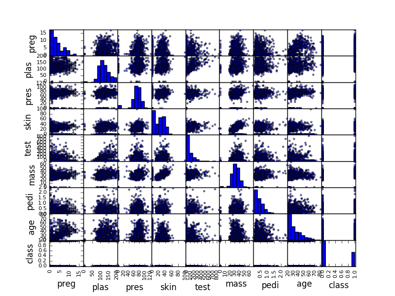
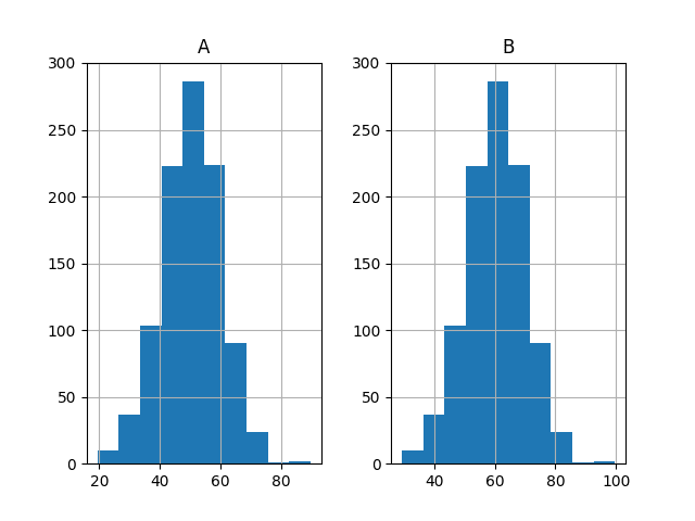
For example, the snippet below will load the diabetes dataset and create a scatterplot matrix of the dataset.

# Scatter Plot Matrix
import matplotlib.pyplot as plt
import pandas
from pandas.tools.plotting import scatter_matrix
url = "https://goo.gl/vhm1eU"
names = ['preg', 'plas', 'pres', 'skin', 'test', 'mass', 'pedi', 'age', 'class']
data = pandas.read_csv(url, names=names)
scatter_matrix(data)
plt.show()

Sample Scatter Plot Matrix

Lesson 6: Prepare For Modeling by Pre-Processing Data

Your raw data may not be setup to be in the best shape for modeling.

Sometimes you need to preprocess your data in order to best present the inherent structure of the problem in your data to the modeling algorithms. In today’s lesson, you will use the pre-processing capabilities provided by the scikit-learn.

The scikit-learn library provides two standard idioms for transforming data. Each transform is useful in different circumstances: Fit and Multiple Transform and Combined Fit-And-Transform.

There are many techniques that you can use to prepare your data for modeling. For example, try out some of the following

• Standardize numerical data (e.g. mean of 0 and standard deviation of 1) using the scale and center options.
• Normalize numerical data (e.g. to a range of 0-1) using the range option.
• Explore more advanced feature engineering such as Binarizing.

For example, the snippet below loads the Pima Indians onset of diabetes dataset, calculates the parameters needed to standardize the data, then creates a standardized copy of the input data.

# Standardize data (0 mean, 1 stdev)
from sklearn.preprocessing import StandardScaler
import pandas
import numpy
url = "https://goo.gl/vhm1eU"
names = ['preg', 'plas', 'pres', 'skin', 'test', 'mass', 'pedi', 'age', 'class']
dataframe = pandas.read_csv(url, names=names)
array = dataframe.values
# separate array into input and output components
X = array[:,0:8]
Y = array[:,8]
scaler = StandardScaler().fit(X)
rescaledX = scaler.transform(X)
# summarize transformed data
numpy.set_printoptions(precision=3)
print(rescaledX[0:5,:])

Lesson 7: Algorithm Evaluation With Resampling Methods

The dataset used to train a machine learning algorithm is called a training dataset. The dataset used to train an algorithm cannot be used to give you reliable estimates of the accuracy of the model on new data. This is a big problem because the whole idea of creating the model is to make predictions on new data.

You can use statistical methods called resampling methods to split your training dataset up into subsets, some are used to train the model and others are held back and used to estimate the accuracy of the model on unseen data.

Your goal with today’s lesson is to practice using the different resampling methods available in scikit-learn, for example:

• Split a dataset into training and test sets.
• Estimate the accuracy of an algorithm using k-fold cross validation.
• Estimate the accuracy of an algorithm using leave one out cross validation.

The snippet below uses scikit-learn to estimate the accuracy of the Logistic Regression algorithm on the Pima Indians onset of diabetes dataset using 10-fold cross validation.

# Evaluate using Cross Validation
import pandas
from sklearn import cross_validation
from sklearn.linear_model import LogisticRegression
url = "https://goo.gl/vhm1eU"
names = ['preg', 'plas', 'pres', 'skin', 'test', 'mass', 'pedi', 'age', 'class']
dataframe = pandas.read_csv(url, names=names)
array = dataframe.values
X = array[:,0:8]
Y = array[:,8]
num_folds = 10
num_instances = len(X)
seed = 7
kfold = cross_validation.KFold(n=num_instances, n_folds=num_folds, random_state=seed)
model = LogisticRegression()
results = cross_validation.cross_val_score(model, X, Y, cv=kfold)
print("Accuracy: %.3f%% (%.3f%%)") % (results.mean()*100.0, results.std()*100.0)

What accuracy did you get? Let me know in the comments.

Did you realize that this is the halfway point? Well done!

Lesson 8: Algorithm Evaluation Metrics

There are many different metrics that you can use to evaluate the skill of a machine learning algorithm on a dataset.

You can specify the metric used for your test harness in scikit-learn via the cross_validation.cross_val_score() function and defaults can be used for regression and classification problems. Your goal with today’s lesson is to practice using the different algorithm performance metrics available in the scikit-learn package.

• Practice using the Accuracy and LogLoss metrics on a classification problem.
• Practice generating a confusion matrix and a classification report.
• Practice using RMSE and RSquared metrics on a regression problem.

The snippet below demonstrates calculating the LogLoss metric on the Pima Indians onset of diabetes dataset.

# Cross Validation Classification LogLoss
import pandas
from sklearn import cross_validation
from sklearn.linear_model import LogisticRegression
url = "https://goo.gl/vhm1eU"
names = ['preg', 'plas', 'pres', 'skin', 'test', 'mass', 'pedi', 'age', 'class']
dataframe = pandas.read_csv(url, names=names)
array = dataframe.values
X = array[:,0:8]
Y = array[:,8]
num_folds = 10
num_instances = len(X)
seed = 7
kfold = cross_validation.KFold(n=num_instances, n_folds=num_folds, random_state=seed)
model = LogisticRegression()
scoring = 'log_loss'
results = cross_validation.cross_val_score(model, X, Y, cv=kfold, scoring=scoring)
print("Logloss: %.3f (%.3f)") % (results.mean(), results.std())

What log loss did you get? Let me know in the comments.

Lesson 9: Spot-Check Algorithms

You cannot possibly know which algorithm will perform best on your data beforehand.

You have to discover it using a process of trial and error. I call this spot-checking algorithms. The scikit-learn library provides an interface to many machine learning algorithms and tools to compare the estimated accuracy of those algorithms.

In this lesson, you must practice spot checking different machine learning algorithms.

• Spot check linear algorithms on a dataset (e.g. linear regression, logistic regression and linear discriminate analysis).
• Spot check some non-linear algorithms on a dataset (e.g. KNN, SVM and CART).
• Spot-check some sophisticated ensemble algorithms on a dataset (e.g. random forest and stochastic gradient boosting).

For example, the snippet below spot-checks the K-Nearest Neighbors algorithm on the Boston House Price dataset.

# KNN Regression
import pandas
from sklearn import cross_validation
from sklearn.neighbors import KNeighborsRegressor
url = "https://goo.gl/sXleFv"
names = ['CRIM', 'ZN', 'INDUS', 'CHAS', 'NOX', 'RM', 'AGE', 'DIS', 'RAD', 'TAX', 'PTRATIO', 'B', 'LSTAT', 'MEDV']
dataframe = pandas.read_csv(url, delim_whitespace=True, names=names)
array = dataframe.values
X = array[:,0:13]
Y = array[:,13]
num_folds = 10
num_instances = len(X)
seed = 7
kfold = cross_validation.KFold(n=num_instances, n_folds=num_folds, random_state=seed)
model = KNeighborsRegressor()
scoring = 'mean_squared_error'
results = cross_validation.cross_val_score(model, X, Y, cv=kfold, scoring=scoring)
print(results.mean())

What mean squared error did you get? Let me know in the comments.

Lesson 10: Model Comparison and Selection

Now that you know how to spot check machine learning algorithms on your dataset, you need to know how to compare the estimated performance of different algorithms and select the best model.

In today’s lesson, you will practice comparing the accuracy of machine learning algorithms in Python with scikit-learn.

• Compare linear algorithms to each other on a dataset.
• Compare nonlinear algorithms to each other on a dataset.
• Compare different configurations of the same algorithm to each other.
• Create plots of the results comparing algorithms.

The example below compares Logistic Regression and Linear Discriminant Analysis to each other on the Pima Indians onset of diabetes dataset.

# Compare Algorithms
import pandas
from sklearn import cross_validation
from sklearn.linear_model import LogisticRegression
from sklearn.discriminant_analysis import LinearDiscriminantAnalysis
# load dataset
url = "https://goo.gl/vhm1eU"
names = ['preg', 'plas', 'pres', 'skin', 'test', 'mass', 'pedi', 'age', 'class']
dataframe = pandas.read_csv(url, names=names)
array = dataframe.values
X = array[:,0:8]
Y = array[:,8]
# prepare configuration for cross validation test harness
num_folds = 10
num_instances = len(X)
seed = 7
# prepare models
models = []
models.append(('LR', LogisticRegression()))
models.append(('LDA', LinearDiscriminantAnalysis()))
# evaluate each model in turn
results = []
names = []
scoring = 'accuracy'
for name, model in models:
	kfold = cross_validation.KFold(n=num_instances, n_folds=num_folds, random_state=seed)
	cv_results = cross_validation.cross_val_score(model, X, Y, cv=kfold, scoring=scoring)
	results.append(cv_results)
	names.append(name)
	msg = "%s: %f (%f)" % (name, cv_results.mean(), cv_results.std())
	print(msg)

Which algorithm got better results? Can you do better? Let me know in the comments.

Lesson 11: Improve Accuracy with Algorithm Tuning

Once you have found one or two algorithms that perform well on your dataset, you may want to improve the performance of those models.

One way to increase the performance of an algorithm is to tune its parameters to your specific dataset.

The scikit-learn library provides two ways to search for combinations of parameters for a machine learning algorithm. Your goal in today’s lesson is to practice each.

• Tune the parameters of an algorithm using a grid search that you specify.
• Tune the parameters of an algorithm using a random search.

The snippet below uses is an example of using a grid search for the Ridge Regression algorithm on the Pima Indians onset of diabetes dataset.

# Grid Search for Algorithm Tuning
import pandas
import numpy
from sklearn import cross_validation
from sklearn.linear_model import Ridge
from sklearn.grid_search import GridSearchCV
url = "https://goo.gl/vhm1eU"
names = ['preg', 'plas', 'pres', 'skin', 'test', 'mass', 'pedi', 'age', 'class']
dataframe = pandas.read_csv(url, names=names)
array = dataframe.values
X = array[:,0:8]
Y = array[:,8]
alphas = numpy.array([1,0.1,0.01,0.001,0.0001,0])
param_grid = dict(alpha=alphas)
model = Ridge()
grid = GridSearchCV(estimator=model, param_grid=param_grid)
grid.fit(X, Y)
print(grid.best_score_)
print(grid.best_estimator_.alpha)

Which parameters achieved the best results? Can you do better? Let me know in the comments.

Lesson 12: Improve Accuracy with Ensemble Predictions

Another way that you can improve the performance of your models is to combine the predictions from multiple models.

Some models provide this capability built-in such as random forest for bagging and stochastic gradient boosting for boosting. Another type of ensembling called voting can be used to combine the predictions from multiple different models together.

In today’s lesson, you will practice using ensemble methods.

• Practice bagging ensembles with the random forest and extra trees algorithms.
• Practice boosting ensembles with the gradient boosting machine and AdaBoost algorithms.
• Practice voting ensembles using by combining the predictions from multiple models together.

The snippet below demonstrates how you can use the Random Forest algorithm (a bagged ensemble of decision trees) on the Pima Indians onset of diabetes dataset.

# Random Forest Classification
import pandas
from sklearn import cross_validation
from sklearn.ensemble import RandomForestClassifier
url = "https://goo.gl/vhm1eU"
names = ['preg', 'plas', 'pres', 'skin', 'test', 'mass', 'pedi', 'age', 'class']
dataframe = pandas.read_csv(url, names=names)
array = dataframe.values
X = array[:,0:8]
Y = array[:,8]
num_folds = 10
num_instances = len(X)
seed = 7
num_trees = 100
max_features = 3
kfold = cross_validation.KFold(n=num_instances, n_folds=num_folds, random_state=seed)
model = RandomForestClassifier(n_estimators=num_trees, max_features=max_features)
results = cross_validation.cross_val_score(model, X, Y, cv=kfold)
print(results.mean())

Can you devise a better ensemble? Let me know in the comments.

Lesson 13: Finalize And Save Your Model

Once you have found a well-performing model on your machine learning problem, you need to finalize it.

In today’s lesson, you will practice the tasks related to finalizing your model.

Practice making predictions with your model on new data (data unseen during training and testing).
Practice saving trained models to file and loading them up again.

For example, the snippet below shows how you can create a Logistic Regression model, save it to file, then load it later and make predictions on unseen data.

# Save Model Using Pickle
import pandas
from sklearn import cross_validation
from sklearn.linear_model import LogisticRegression
import pickle
url = "https://goo.gl/vhm1eU"
names = ['preg', 'plas', 'pres', 'skin', 'test', 'mass', 'pedi', 'age', 'class']
dataframe = pandas.read_csv(url, names=names)
array = dataframe.values
X = array[:,0:8]
Y = array[:,8]
test_size = 0.33
seed = 7
X_train, X_test, Y_train, Y_test = cross_validation.train_test_split(X, Y, test_size=test_size, random_state=seed)
# Fit the model on 33%
model = LogisticRegression()
model.fit(X_train, Y_train)
# save the model to disk
filename = 'finalized_model.sav'
pickle.dump(model, open(filename, 'wb'))

# some time later...

# load the model from disk
loaded_model = pickle.load(open(filename, 'rb'))
result = loaded_model.score(X_test, Y_test)
print(result)

Lesson 14: Hello World End-to-End Project

You now know how to complete each task of a predictive modeling machine learning problem.

In today’s lesson, you need to practice putting the pieces together and working through a standard machine learning dataset end-to-end.

Work through the iris dataset end-to-end (the hello world of machine learning)

This includes the steps:

1. Understanding your data using descriptive statistics and visualization.
2. Preprocessing the data to best expose the structure of the problem.
3. Spot-checking a number of algorithms using your own test harness.
4. Improving results using algorithm parameter tuning.
5. Improving results using ensemble methods.
6. Finalize the model ready for future use.

Take it slowly and record your results along the way.

What model did you use? What results did you get? Let me know in the comments.

The End!
(Look How Far You Have Come)

You made it. Well done!

Take a moment and look back at how far you have come.

• You started off with an interest in machine learning and a strong desire to be able to practice and apply machine learning using Python.
• You downloaded, installed and started Python, perhaps for the first time and started to get familiar with the syntax of the language.
• Slowly and steadily over the course of a number of lessons you learned how the standard tasks of a predictive modeling machine learning project map onto the Python platform.
• Building upon the recipes for common machine learning tasks you worked through your first machine learning problems end-to-end using Python.
• Using a standard template, the recipes and experience you have gathered you are now capable of working through new and different predictive modeling machine learning problems on your own.

Don’t make light of this, you have come a long way in a short amount of time.

This is just the beginning of your machine learning journey with Python. Keep practicing and developing your skills.

Summary

How Did You Go With The Mini-Course?
Did you enjoy this mini-course?

Do you have any questions? Were there any sticking points?
Let me know. Leave a comment below.

Frustrated With Python Machine Learning?

Develop Your Own Models and Predictions in Minutes

...with just a few lines of scikit-learn code

Discover how in my new Ebook: Machine Learning Mastery With Python

It covers self-study tutorials and end-to-end projects on topics like:
Loading data, visualization, modeling, algorithm tuning, and much more...

Finally Bring Machine Learning To
Your Own Projects

Skip the Academics. Just Results.

Click to learn more.

The post Python Machine Learning Mini-Course appeared first on Machine Learning Mastery.

You should pick the right tool for the job.

The specific predictive modeling problem that you are working on should dictate the specific programming language, libraries and even machine learning algorithms to use.

But, what if you are just getting started and looking for a platform to learn and practice machine learning?

In this post, you will discover that Python is the growing platform for applied machine learning, likely to outpace and topple R in terms of adoption and perhaps capability.

After reading this post you will know:

• That search volume for Python machine learning is growing fast and has already outpaced R.
• That the percentage of Python machine learning jobs is growing and has already outpaced R.
• That Python is used by nearly 50% of polled practitioners and growing.

Let’s get started.

Python for Machine Learning is Growing

Let’s look at 3 areas where we can see Python for machine learning growing:

1. Search Volume.
2. Job Ads.
3. Professional Tool Usage.

Python Machine Learning Search Volume is Growing

Search volume is probably indicative of students, engineers and other practitioners searching for information to get started or go deeper into the topic.

Google provides a tool called Google Trends that gives insight into the search volume of keywords over time.

We can investigate the growth of “Python machine learning” from 2004 to 2016 (the last 12 years). Below is a graph of the change in search volume for this period:

Growth in Search Traffic for Python Machine Learning

We can see that the trend upward started in Perhaps 2012 with a steeper rise starting in 2015, likely boosted by Python Deep Learning tools like TensorFlow.

We can also contrast this to the search volume for R machine learning and we can see that from about the middle of 2015, Python machine learning has been beating out R.

Python Machine Learning vs R Machine Learning Search Volume

Blue denotes “Python Machine Learning” and red denotes “R Machine Learning”.

Python Machine Learning Jobs are Growing

Indeed is a job search website and like Google trends, they show the volume of job ads that match keywords.

We can investigate the demand for “python machine learning jobs” for the last 4 years.

Growth on Python Machine Learning Jobs

We can see time along the x-axis and the percentage of job postings that match the keyword. The graph shows almost linear growth from 2012 to 2015 with a hockey-stick like increase in 2016.

We can also compare the job ads for python and R.

Python Machine Learning Jobs vs R Machine Learning Jobs

Blue shows “Python machine learning” and orange shows “R machine learning”.

We see a more pronounced story compared to Google search volume. The percentage of job ads available to indeed.com shows that demand for Python machine learning skills has been dominating R machine learning skills since at least 2012 with the gap only widening in recent years.

KDNuggets Survey Results: More People Using Python for Machine Learning

We can get some insight into the tools used by machine learning practitioners by reviewing the results for the KDnuggets Software Poll Results.

Here’s a quote from the 2016 results:

R remains the leading tool, with 49% share, but Python grows faster and almost catches up to R.

— Gregory Piatetsky

The poll tracks the tools used by machine learning and data science professionals, where a participant can select more than one tool (which is the norm I would expect)

Here is the growth of Python for machine learning over the last 4 years:

2016   45.8%
2015   30.3%
2014   19.5%
2013   13.3%

Below is a plot of this growth.

KDNuggets Poll Results – Percentage of Professionals Using Python.png

We can see a near linear growth trend where Python s used by just under 50% of profesionals in 2016.

It is important to note that the number of participants in the poll has also grown from many hundreds to thousands in recent years and participants are self-selected.

What is interesting is that scikit-learn also appears separately on the poll, accounting for 17.2%.

For more information see: KDnuggets 2016 Software Poll Results.

O’Reilly Survey Results: More People Using Python for Machine Learning

O’Reilly performs an annual Data Science Salary Survey.

They collect a lot of data from professional data scientists and machine learning practitioners and present the results in very nice reports. For example, here is the 2016 Data Science Salary Survey report [View the PDF Report].

The survey tracks tool usage of practitioners, and as with the KDNuggets data.

Quoting from the key findings from the 2016 report, we can see that Python plays an important role in data science salary.

Python and Spark are among the tools that contribute most to salary.

— Page 1, 2016 Data Science Salary Survey report.

Reviewing the survey results, we can see a similar growth trend in use of the use of the Python ecosystem for machine learning over the last 4 years.

2016   54%
2015   51%
2014   42% (interpreted from graph)
2013   40%

Again, we can plot this growth.

O’Reilly Poll Results – Percentage of Professionals Using Python.png

It’s interesting that the 2016 results are very similar to those from the KDNuggets poll.

Quotes

You can find quotes to support any position on the Internet.

Take quotes with a grain of salt. Nevertheless, quotes can be insightful, raising and supporting points.

Let’s first take a look at some cherry-picked quotes from news sites and blogs about the growth of Python for machine learning.

News Quotes

Python has emerged over the past few years as a leader in data science programming. While there are still plenty of folks using R, SPSS, Julia or several other popular languages, Python’s growing popularity in the field is evident in the growth of its data science libraries.

— Katharine Jarmul, Introduction To Data Science: How To “big Data” With Python, Dataconomy

Our research shows that Python is one of the most popular languages for data science analyses, in use by more than one-third (36%) of organizations.

— Dave Menninger, Big Data Grows Up at Strata+Hadoop World 2016, SmartDataCollective

… the last few years have seen a proliferation of cutting-edge, commercially usable machine learning frameworks, including the highly successful scikit-learn Python library and well-publicized releases of libraries like Tensorflow by Google and CNTK by Microsoft Research.

— Josh Schwartz, Machine Learning Is No Longer Just for Experts, Harvard Business Review

Note that scikit-learn, TensorFlow and CNTK are all Python machine learning libraries.

Python is versatile, simple, easier to learn, and powerful because of its usefulness in a variety of contexts, some of which have nothing to do with data science. R is a specialized environment that looks to optimize for data analysis, but which is harder to learn. You’ll get paid more if you stick it out with R rather than working with Python

— Roger Huang, Data science sexiness: Your guide to Python and R, and which one is best, TheNextWeb

Quora Quotes

Below are some cherry picked quotes regarding the use of Python for machine learning taken from Quora questions.

Python if a popular scientific language and a rising star for machine learning. I’d be surprised if it can take the data analysis mantle from R, but matrix handling in NumPy may challenge MATLAB and communication tools like IPython are very attractive and a step into the future of reproducibility. I think the SciPy stack for machine learning and data analysis can be used for one-off projects (like papers), and frameworks like scikit-learn may be mature enough to be used in production systems.

— Aswath Muralidharan, Production Engineer. In response to the Quora question “What are the top 5 programming languages for Machine Learning?”

I’d also recommend Python as it is a fantastic all-round programming language that is incredibly useful for drafting code fragments and exploring data (with the IPython shell), great for documenting steps and results in the analytical process chain (IPython Notebook), has a huge selection of libraries for almost any machine learning objective and can even be optimized for production system implementation. In my opinions there are languages that are superior to Python in any of these categories – but none of them offers this versatility.

— Benedikt Koehler, Founder & CEO DataLion. In response to the Quora question “What is the best language to use while learning machine learning for the first time?”

[…] It is because the language can make a productive environment for people that just want to get something done quickly. It is fairly easy to wrap C libraries, and C++ is doable. This gives Python access to a wide range of existing code. Also the language doesn’t get in the way when it comes time to implement things. In many ways it makes coding “fun again” for a wide range of tasks.

— Shawn Masters, VP of Engineering. In response to the Quora question “Will Python become as popular as Java, given that Python is used in Machine Learning?”

In my opinion, Python truly dominates this category. A quick search of almost any artificial intelligence, machine learning, NLP, or data analytics topic, plus ‘Python’, will return examples of useful, actively maintained libraries.

— Ryan Hill, programmer. In response to the Quora question “Which programming language has the best repository of machine learning libraries?”

Summary

In this post, you discovered that Python is the growing platform for applied machine learning.

Specifically, you learned that:

• The number of people interested in Python for machine learning is larger than R and is growing.
• The number of jobs posted for Python machine learning skills is larger than R and growing.
• The number of polled data science professionals that use Python is growing year over year.

Has this influenced your decision to get started with the
Python ecosystem for machine learning?
Share your thoughts in the comments below.

The post Python is the Growing Platform for Applied Machine Learning appeared first on Machine Learning Mastery.

Linux is an excellent environment for machine learning development with Python.

The tools can be installed quickly and easily and you can develop and run large models directly.

In this tutorial, you will discover how to create and setup a Linux virtual machine for machine learning with Python.

After completing this tutorial, you will know:

• How to download and install VirtualBox for managing virtual machines.
• How to download and setup Fedora Linux.
• How to install a SciPy environment for machine learning in Python 3.

This tutorial is suitable if your base operating system is Windows, Mac OS X, and Linux.

Let’s get started.

Benefits of a Linux Virtual Machine

There are a number of reasons that you may want to use a Linux virtual machine for Python machine learning development.

For example, below is a list of 5 top benefits for using a virtual machine:

• To use tools not available on your system (if you’re on Windows).
• To install and use machine learning tools without impacting your local environment (e.g. use Python 3 tools).
• To have highly customized environments for different projects (Python2 and Python3).
• To save the state of the machine and pick up exactly where you left off (jump from machine to machine).
• To share development environment with other developers (set-up once and reuse many times).

Perhaps the most beneficial point is the first, being able to easily use machine learning tools not supported on your environment.

I’m an OS X user, and even though machine learning tools can be installed using brew and macports, I still find it easier to setup and use Linux virtual machines for machine learning development.

Overview

This tutorial is broken down into 3 parts:

1. Download and Install VirtualBox.
2. Download and Install Fedora Linux in a Virtual Machine.
3. Install Python Machine Learning Environment

1. Download and Install VirtualBox

VirtualBox is a free open source platform for creating and managing virtual machines.

Once installed, you can create all the virtual machines you like, as long as you have the ISO images or CDs to install from.

• 1. Visit VirtualBox.org
• 2. Click “Download VirtualBox” to access the Downloads page.

Download VirtualBox

• 3. Choose binaries for your workstation.
• 4. Install the software for your system and follow the installation instructions.

Install VirtualBox

• 5. Open the VirtualBox software and confirm it works.

Start VirtualBox

2. Download and Install Fedora Linux

I chose Fedora Linux because I think it is a kinder and gentler Linux than some.

It is a leading edge for RedHat Linux intended for workstations and developers.

2.1 Download the Fedora ISO Image

Let’s start off by downloading the ISO for Fedora Linux. In this case, the 64-bit version of Fedora 25.

• 1. Visit GetFedora.org.
• 2. Click “Workstation” to access the Workstation page.
• 3. Click “Download now” to access the Downloads page.
• 4. Under “Other Downloads” click “64-bit 1.3GB Live image“

Download Fedora

• 5. You should now have an ISO file with the name:
  • “Fedora-Workstation-Live-x86_64-25-1.3.iso“.

We are now ready to create the VM in VirtualBox.

2.2 Create the Fedora Virtual Machine

Now, let’s create the Fedora virtual machine in VirtualBox.

• 1. Open the VirtualBox software.
• 2. Click “New” button.
• 3. Select the Name and operating system.
  • name: Fedora25
  • type: Linux
  • version: Fedora (64-bit)
  • Click “Continue“

Create Fedora VM Name and Operating System

• 4. Configure the Memory Size
  • 2048
• 5. Configure the Hard Disk
  • Create a virtual hard disk now
  • Hard disk file type
  • VDI (VirtualBox Disk Image)
  • Storage on physical hard disk
  • Dynamically allocated
  • File location and size: 10GB

We are now ready to install Fedora from the ISO image.

2.3 Install Fedora Linux

Now, let’s install Fedora Linux on the new virtual machine.

• 1. Select the new virtual machine and click the “Start” button.
• 2. Click Folder Icon and choose the Fedora ISO file:
  • “Fedora-Workstation-Live-x86_64-25-1.3.iso“.

Install Fedora

• 3. Click the “Start” button.
• 4. Select the first option “Start Fedora-Live-Workstation-Live 25” and press the Enter key.
• 5. Hit the “Esc” key to skip the check.
• 6. Select “Live System User“.
• 7. Select “Install to Hard Drive“.

Install Fedora to Hard Drive

• 8. Complete “Language Selection” (English)
• 9. Complete “Installation Destination” (“ATA VBOX HARDDISK“).
  • You may need to wait one minute for the VM to create the hard disk.

Install on Virtual Hard Disk

• 10. Click “Begin Installation“.
• 11. Set root password.
• 12. Create a user for yourself.
  • Note down the username and password (so that you can use it later).
  • Tick the “Make this user administrator” (so you can install software).

Create a New User

• 13. Wait for the installation to complete… (5 minutes?)
• 14. Click “Quit”, click power icon in top right; select power off.

2.4 Finalize Fedora Linux Installation

Fedora Linux has been installed; let’s finalize the installation and make it ready for use.

• 1. In VirtualBox with the Fedora25 VM selected, under “Storage“, click on “Optical Drive“.
  • Select “Remove disk from virtual drive” to eject the ISO image.
• 2. Click the “Start” button to start the Fedora Linux installation.
• 3. Login as the user you created.

Fedora Login as New User

• 4. Finalize installation
  • Choose language “English“
  • Click “Next“
  • Choose Keyboard “US“
  • Click “Next“
  • Configure Privacy
  • Click “Next“
  • Connect Your Online Accounts
  • Click “Skip“
  • Click “Start using Fedora“
• 5. Close the help system that starts automatically.

We now have a Fedora Linux virtual machine ready to install new software.

3. Install Python Machine Learning Environment

Fedora uses Gnome 3 as the window manager.

Gnome 3 is quite different to prior versions of Gnome; you can learn how to get around by using the built-in help system.

3.1 Install Python Environment

Let’s start off by installing the required Python libraries for machine learning development.

• 1. Open the terminal.
  • Click “Activities“
  • Type “terminal“
  • Click icon or press enter

Start Terminal

• 2. Confirm Python3 was installed.

Type:

python3 --version

Python3 Version

• 3. Install the Python machine learning environment. Specifically:
  • NumPy
  • SciPy
  • Pandas
  • Matplotlib
  • Statsmodels
  • Scikit-Learn

DNF is the software installation system, formally yum. The first time you run dnf, it will update the database of packages, this might take a minute.

Type:

sudo dnf install python3-numpy python3-scipy python3-scikit-learn python3-pandas python3-matplotlib python3-statsmodels

Enter your password when prompted.

Confirm the installation when prompted by pressing “y” and “enter“.

3.2 Confirm Python Environment

Now that the environment is installed, we can confirm it by printing the versions of each required library.

• 1. Open Gedit.
  • Click “Activities“
  • Type “gedit“
  • Click icon or press enter
• 2. Type the following script and save it as versions.py in the home directory.

# scipy
import scipy
print('scipy: %s' % scipy.__version__)
# numpy
import numpy
print('numpy: %s' % numpy.__version__)
# matplotlib
import matplotlib
print('matplotlib: %s' % matplotlib.__version__)
# pandas
import pandas
print('pandas: %s' % pandas.__version__)
# scikit-learn
import sklearn
print('sklearn: %s' % sklearn.__version__)
# statsmodels
import statsmodels
print('statsmodels: %s' % statsmodels.__version__)

There is no copy-paste support; you may want to open Firefox within the VM and navigate to this page and copy paste the script into your Gedit window.

Write Versions Script

• 3. Run the script in the terminal.

Type:

python3 versions.py

Python3 Check Library Versions

Tips For Using the VM

This section lists some tips using the VM for machine learning development.

• Copy-paste and Folder Sharing. These features require the installation of “Guest Additions” in the Linux VM. I have not been able to get this to install correctly and therefore do not use these features. You can try if you like; let me know how you do in the comments.
• Use GitHub. I recommend storing all of your code in GitHub and checking the code in and out from the VM. It makes life a lot easier for getting code and assets in and out of the VM.
• Use Sublime. I think sublime is a great text editor on Linux for development, better than Gedit at least.
• Use AWS for large jobs. You can use the same procedure to setup Fedora Linux on Amazon Web Services for running large models in the cloud.
• VM Tools. You can save the VM at any point by closing the window. You can also take a snapshot of the VM at any point and return to the snapshot. This can be helpful if you are making large changes to the file system.
• Python2. You can easily install Python2 alongside Python 3 in Linux and use the python (rather than python3) binary or use alternatives to switch between the two.
• Notebooks. Consider running a notebook server inside the VM and opening up the firewall so that you can connect and run from your main workstation outside of the VM.

Do you have any tips to share? Let me know in the comments.

Further Reading

Below are some resources for further reading if you are new to the tools used in this tutorial.

• VirtualBox User Manual
• Fedora Documentation
• Fedora Wiki (tons of help on common topics)
• SciPy Homepage
• Scikit-Learn Homepage

Summary

In this tutorial, you discovered how to setup a Linux virtual machine for Python machine learning development.

Specifically, you learned:

• How to download and install VirtualBox, free, open-source software for managing virtual machines.
• How to download and setup Fedora Linux, a friendly Linux distribution for developers.
• How to install and test a Python3 environment for machine learning development.

Did you complete the tutorial?
Let me know how it went in the comments below.

The post How to Create a Linux Virtual Machine For Machine Learning Development With Python 3 appeared first on Machine Learning Mastery.

It can be difficult to install a Python machine learning environment on some platforms.

Python itself must be installed first and then there are many packages to install, and it can be confusing for beginners.

In this tutorial, you will discover how to set up a Python machine learning development environment using Anaconda.

After completing this tutorial, you will have a working Python environment to begin learning, practicing, and developing machine learning and deep learning software.

These instructions are suitable for Windows, Mac OS X, and Linux platforms. I will demonstrate them on OS X, so you may see some mac dialogs and file extensions.

How to Setup a Python Environment for Machine Learning and Deep Learning with Anaconda

Overview

In this tutorial, we will cover the following steps:

1. Download Anaconda
2. Install Anaconda
3. Start and Update Anaconda
4. Update scikit-learn Library
5. Install Deep Learning Libraries

1. Download Anaconda

In this step, we will download the Anaconda Python package for your platform.

Anaconda is a free and easy-to-use environment for scientific Python.

• 1. Visit the Anaconda homepage.
• 2. Click “Anaconda” from the menu and click “Download” to go to the download page.

Click Anaconda and Download

• 3. Choose the download suitable for your platform (Windows, OSX, or Linux):
  • Choose Python 3.5
  • Choose the Graphical Installer

Choose Anaconda Download for Your Platform

This will download the Anaconda Python package to your workstation.

I’m on OS X, so I chose the OS X version. The file is about 426 MB.

You should have a file with a name like:

Anaconda3-4.2.0-MacOSX-x86_64.pkg

2. Install Anaconda

In this step, we will install the Anaconda Python software on your system.

This step assumes you have sufficient administrative privileges to install software on your system.

• 1. Double click the downloaded file.
• 2. Follow the installation wizard.

Anaconda Python Installation Wizard

Installation is quick and painless.

There should be no tricky questions or sticking points.

Anaconda Python Installation Wizard Writing Files

The installation should take less than 10 minutes and take up a little more than 1 GB of space on your hard drive.

3. Start and Update Anaconda

In this step, we will confirm that your Anaconda Python environment is up to date.

Anaconda comes with a suite of graphical tools called Anaconda Navigator. You can start Anaconda Navigator by opening it from your application launcher.

Anaconda Navigator GUI

You can learn all about the Anaconda Navigator here.

You can use the Anaconda Navigator and graphical development environments later; for now, I recommend starting with the Anaconda command line environment called conda.

Conda is fast, simple, it’s hard for error messages to hide, and you can quickly confirm your environment is installed and working correctly.

• 1. Open a terminal (command line window).
• 2. Confirm conda is installed correctly, by typing:

conda -V

You should see the following (or something similar):

conda 4.2.9

• 3. Confirm Python is installed correctly by typing:

python -V

You should see the following (or something similar):

Python 3.5.2 :: Anaconda 4.2.0 (x86_64)

Confirm Conda and Python are Installed

If the commands do not work or have an error, please check the documentation for help for your platform.

See some of the resources in the “Further Reading” section.

• 4. Confirm your conda environment is up-to-date, type:

conda update conda
conda update anaconda

You may need to install some packages and confirm the updates.

• 5. Confirm your SciPy environment.

The script below will print the version number of the key SciPy libraries you require for machine learning development, specifically: SciPy, NumPy, Matplotlib, Pandas, Statsmodels, and Scikit-learn.

You can type “python” and type the commands in directly. Alternatively, I recommend opening a text editor and copy-pasting the script into your editor.

# scipy
import scipy
print('scipy: %s' % scipy.__version__)
# numpy
import numpy
print('numpy: %s' % numpy.__version__)
# matplotlib
import matplotlib
print('matplotlib: %s' % matplotlib.__version__)
# pandas
import pandas
print('pandas: %s' % pandas.__version__)
# statsmodels
import statsmodels
print('statsmodels: %s' % statsmodels.__version__)
# scikit-learn
import sklearn
print('sklearn: %s' % sklearn.__version__)

Save the script as a file with the name: versions.py.

On the command line, change your directory to where you saved the script and type:

python versions.py

You should see output like the following:

scipy: 0.18.1
numpy: 1.11.1
matplotlib: 1.5.3
pandas: 0.18.1
statsmodels: 0.6.1
sklearn: 0.17.1

What versions did you get?
Paste the output in the comments below.

Confirm Anaconda SciPy environment

4. Update scikit-learn Library

In this step, we will update the main library used for machine learning in Python called scikit-learn.

• 1. Update scikit-learn to the latest version.

At the time of writing, the version of scikit-learn shipped with Anaconda is out of date (0.17.1 instead of 0.18.1). You can update a specific library using the conda command; below is an example of updating scikit-learn to the latest version.

At the terminal, type:

conda update scikit-learn

Update scikit-learn in Anaconda

Alternatively, you can update a library to a specific version by typing:

conda install -c anaconda scikit-learn=0.18.1

Confirm the installation was successful and scikit-learn was updated by re-running the versions.py script by typing:

python versions.py

You should see output like the following:

scipy: 0.18.1
numpy: 1.11.3
matplotlib: 1.5.3
pandas: 0.18.1
statsmodels: 0.6.1
sklearn: 0.18.1

What versions did you get?
Paste the output in the comments below.

You can use these commands to update machine learning and SciPy libraries as needed.

Try a scikit-learn tutorial, such as:

• Your First Machine Learning Project in Python Step-By-Step

5. Install Deep Learning Libraries

In this step, we will install Python libraries used for deep learning, specifically: Theano, TensorFlow, and Keras.

• 1. Install the Theano deep learning library by typing:

conda install theano

• 2. Install the TensorFlow deep learning library (all except Windows) by typing:

conda install -c conda-forge tensorflow

Alternatively, you may choose to install using pip and a specific version of tensorflow for your platform.

See the installation instructions for tensorflow.

• 3. Install Keras by typing:

pip install keras

• 4. Confirm your deep learning environment is installed and working correctly.

Create a script that prints the version numbers of each library, as we did before for the SciPy environment.

# theano
import theano
print('theano: %s' % theano.__version__)
# tensorflow
import tensorflow
print('tensorflow: %s' % tensorflow.__version__)
# keras
import keras
print('keras: %s' % keras.__version__)

Save the script to a file deep_versions.py. Run the script by typing:

python deep_versions.py

You should see output like:

theano: 0.8.2.dev-901275534cbfe3fbbe290ce85d1abf8bb9a5b203
tensorflow: 0.12.1
Using TensorFlow backend.
keras: 1.2.1

Anaconda Confirm Deep Learning Libraries

What versions did you get?
Paste your output in the comments below.

Try a Keras deep learning tutorial, such as:

• Develop Your First Neural Network in Python With Keras Step-By-Step

Further Reading

This section provides some links for further reading.

• Anaconda Documentation
• Anaconda Documentation: Installation
• Conda
• Using conda
• Anaconda Navigator
• Installing Theano
• Install TensorFlow Anaconda
• Keras Installation

Summary

Congratulations, you now have a working Python development environment for machine learning and deep learning.

You can now learn and practice machine learning and deep learning on your workstation.

How did you go?
Let me know in the comments below.

The post How to Setup a Python Environment for Machine Learning and Deep Learning with Anaconda appeared first on Machine Learning Mastery.

It can be difficult to install a Python machine learning environment on Mac OS X.

Python itself must be installed first, and then there are many packages to install, and it can be confusing for beginners.

In this tutorial, you will discover how to setup a Python 3 machine learning and deep learning development environment using macports.

After completing this tutorial, you will have a working Python 3 environment to begin learning, practicing, and developing machine learning and deep learning software.

Let’s get started.

How to Install a Python 3 Environment on Mac OS X for Machine Learning and Deep Learning

Tutorial Overview

This tutorial is broken down into the following 4 steps:

1. Install XCode Tools
2. Install Macports
3. Install SciPy Libraries
4. Install Deep Learning Libraries

1. Install XCode

XCode is the IDE for development on OS X.

Installation of XCode is required because it contains command line tools needed for Python development. In this step, you will install XCode and the XCode command line tools.

This step assumes you already have an Apple App Store account and that you have sufficient administrative privileges to install software on your workstation.

• 1. Open the “App Store” application. Search for “XCode” and click the “Get” button to install.

You will be prompted to enter your App Store password.

XCode is free and is at least 4.5 GB in size and may take some time to download.

App Store Search for XCode

• 2. Open “Applications” and then locate and start “XCode“.

You may be prompted with a message to install additional components before XCode can be started. Agree and install.

Install Additional XCode Components

• 3. Install the XCode Command Line Tools, Open a terminal window and type:

xcode-select --install

A dialog will appear and install required tools.

Confirm the tools are installed by typing:

xcode-select -p

You should see output like:

/Applications/Xcode.app/Contents/Developer

• 4. Agree to the license agreement (if needed). Open a terminal window and type:

xcodebuild -license

Use the “space” key to navigate to the bottom and agree.

You now have XCode and the XCode Command Line Tools installed.

2. Install Macports

Macports is a package management tool for installing development tools on OS X.

In this step, you will install the macports package management tool.

• 1. Visit macports.org
• 2. Click the “Download” button at the top of the page to access the install page.
• 3. Download the “macOS Package (.pkg) Installer” for your version of OS X.

At the time of writing, the latest version of OS X is Sierra.

Macports Package Installation

You should now have a package on your workstation. For example:

MacPorts-2.3.5-10.12-Sierra.pkg

• 4. Double click the package and follow through the wizard to install macports.

Macports Installation Wizard

• 5. Update macports and confirm the system is working as expected. Open a terminal window and type:

sudo port selfupdate

This will update the port command and the list of available ports and is useful to do from time to time.

You should see a message like:

MacPorts base is already the latest version

3. Install SciPy and Machine Learning Libraries

SciPy is the collection of scientific computing Python libraries needed for machine learning development in Python.

In this step, you will install the Python 3 and SciPy environment.

• 1. Install Python version 3.5 using macports. Open a terminal and type:

sudo port install python35

To make this the default version of Python, type:

sudo port select --set python python35
sudo port select --set python3 python35

Close the terminal window and reopen it.

Confirm that Python 3.5 is now the default Python for the system by typing:

python -V

You should see the message below, or similar:

Python 3.5.3

• 2. Install the SciPy environment, including the libraries:
  • NumPy
  • SciPy
  • Matplotlib
  • Pandas
  • Statsmodels
  • Pip (package manager)

Open a terminal and type:

sudo port install py35-numpy py35-scipy py35-matplotlib py35-pandas py35-statsmodels py35-pip

This may take some time to download and install.

To ensure pip for Python 3 is the default for the system, type:

sudo port select --set pip pip35

• 3. Install scikit-learn using pip. Open the command line and type:

sudo pip install -U scikit-learn

• 4. Confirm the libraries were installed correctly. Open a text editor and write (copy-paste) the following script:

# scipy
import scipy
print('scipy: %s' % scipy.__version__)
# numpy
import numpy
print('numpy: %s' % numpy.__version__)
# matplotlib
import matplotlib
print('matplotlib: %s' % matplotlib.__version__)
# pandas
import pandas
print('pandas: %s' % pandas.__version__)
# statsmodels
import statsmodels
print('statsmodels: %s' % statsmodels.__version__)
# scikit-learn
import sklearn
print('sklearn: %s' % sklearn.__version__)

Save the script with the filename versions.py.

Change directory to the location where you saved the script and type:

python versions.py

The output should look like the following (or similar):

scipy: 0.18.1
numpy: 1.12.0
matplotlib: 2.0.0
pandas: 0.19.2
statsmodels: 0.6.1
sklearn: 0.18.1

What versions did you get?
Paste the output in the comments below.

You can use these commands to update machine learning and SciPy libraries as needed.

Try a scikit-learn tutorial, such as:

• Your First Machine Learning Project in Python Step-By-Step

4. Install Deep Learning Libraries

In this step, we will install Python libraries used for deep learning, specifically: Theano, TensorFlow, and Keras.

• 1. Install the Theano deep learning library by typing:

sudo pip install theano

• 2. Install the TensorFlow deep learning library by typing:

sudo pip install tensorflow

• 3. To install Keras, type:

sudo pip install keras

• 4. Confirm your deep learning environment is installed and working correctly.

Create a script that prints the version numbers of each library, as we did before for the SciPy environment.

# theano
import theano
print('theano: %s' % theano.__version__)
# tensorflow
import tensorflow
print('tensorflow: %s' % tensorflow.__version__)
# keras
import keras
print('keras: %s' % keras.__version__)

Save the script to a file deep_versions.py.

Run the script by typing:

python deep_versions.py

You should see output like:

theano: 0.8.2
tensorflow: 0.12.1
Using TensorFlow backend.
keras: 1.2.1

What versions did you get?
Paste the output in the comments below.

Try a Keras deep learning tutorial, such as:

• Develop Your First Neural Network in Python With Keras Step-By-Step

Further Reading

This section provides some resources for further reading.

• MacPorts Installation
• Chapter 2. Installing MacPorts
• Chapter 3. Using MacPorts
• Installing the SciPy Stack
• Scikit-learn Installation
• Installing Theano
• Install TensorFlow Anaconda
• Keras Installation

Summary

Congratulations, you now have a working Python development environment on Mac OS X for machine learning and deep learning.

You can now learn and practice machine learning and deep learning on your workstation.

How did you do?
Let me know in the comments below.

The post How to Install a Python 3 Environment on Mac OS X for Machine Learning and Deep Learning appeared first on Machine Learning Mastery.

Real-world data often has missing values.

Data can have missing values for a number of reasons such as observations that were not recorded and data corruption.

Handling missing data is important as many machine learning algorithms do not support data with missing values.

In this tutorial, you will discover how to handle missing data for machine learning with Python.

Specifically, after completing this tutorial you will know:

• How to marking invalid or corrupt values as missing in your dataset.
• How to remove rows with missing data from your dataset.
• How to impute missing values with mean values in your dataset.

Let’s get started.

Note: The examples in this post assume that you have Python 2 or 3 with Pandas, NumPy and Scikit-Learn installed, specifically scikit-learn version 0.18 or higher.

How to Handle Missing Values with Python
Photo by CoCreatr, some rights reserved.

Overview

This tutorial is divided into 6 parts:

1. Pima Indians Diabetes Dataset: where we look at a dataset that has known missing values.
2. Mark Missing Values: where we learn how to mark missing values in a dataset.
3. Missing Values Causes Problems: where we see how a machine learning algorithm can fail when it contains missing values.
4. Remove Rows With Missing Values: where we see how to remove rows that contain missing values.
5. Impute Missing Values: where we replace missing values with sensible values.
6. Algorithms that Support Missing Values: where we learn about algorithms that support missing values.

First, let’s take a look at our sample dataset with missing values.

1. Pima Indians Diabetes Dataset

The Pima Indians Diabetes Dataset involves predicting the onset of diabetes within 5 years in Pima Indians given medical details.

It is a binary (2-class) classification problem. The number of observations for each class is not balanced. There are 768 observations with 8 input variables and 1 output variable. The variable names are as follows:

• 0. Number of times pregnant.
• 1. Plasma glucose concentration a 2 hours in an oral glucose tolerance test.
• 2. Diastolic blood pressure (mm Hg).
• 3. Triceps skinfold thickness (mm).
• 4. 2-Hour serum insulin (mu U/ml).
• 5. Body mass index (weight in kg/(height in m)^2).
• 6. Diabetes pedigree function.
• 7. Age (years).
• 8. Class variable (0 or 1).

The baseline performance of predicting the most prevalent class is a classification accuracy of approximately 65%. Top results achieve a classification accuracy of approximately 77%.

A sample of the first 5 rows is listed below.

6,148,72,35,0,33.6,0.627,50,1
1,85,66,29,0,26.6,0.351,31,0
8,183,64,0,0,23.3,0.672,32,1
1,89,66,23,94,28.1,0.167,21,0
0,137,40,35,168,43.1,2.288,33,1

This dataset is known to have missing values.

Specifically, there are missing observations for some columns that are marked as a zero value.

We can corroborate this by the definition of those columns and the domain knowledge that a zero value is invalid for those measures, e.g. a zero for body mass index or blood pressure is invalid.

Download the dataset from here and save it to your current working directory with the file name pima-indians-diabetes.csv.

2. Mark Missing Values

In this section, we will look at how we can identify and mark values as missing.

We can use plots and summary statistics to help identify missing or corrupt data.

We can load the dataset as a Pandas DataFrame and print summary statistics on each attribute.

from pandas import read_csv
dataset = read_csv('pima-indians-diabetes.csv', header=None)
print(dataset.describe())

Running this example produces the following output:

0           1           2           3           4           5  \
count  768.000000  768.000000  768.000000  768.000000  768.000000  768.000000
mean     3.845052  120.894531   69.105469   20.536458   79.799479   31.992578
std      3.369578   31.972618   19.355807   15.952218  115.244002    7.884160
min      0.000000    0.000000    0.000000    0.000000    0.000000    0.000000
25%      1.000000   99.000000   62.000000    0.000000    0.000000   27.300000
50%      3.000000  117.000000   72.000000   23.000000   30.500000   32.000000
75%      6.000000  140.250000   80.000000   32.000000  127.250000   36.600000
max     17.000000  199.000000  122.000000   99.000000  846.000000   67.100000

                6           7           8
count  768.000000  768.000000  768.000000
mean     0.471876   33.240885    0.348958
std      0.331329   11.760232    0.476951
min      0.078000   21.000000    0.000000
25%      0.243750   24.000000    0.000000
50%      0.372500   29.000000    0.000000
75%      0.626250   41.000000    1.000000
max      2.420000   81.000000    1.000000

This is useful.

We can see that there are columns that have a minimum value of zero (0). On some columns, a value of zero does not make sense and indicates an invalid or missing value.

Specifically, the following columns have an invalid zero minimum value:

• 1: Plasma glucose concentration
• 2: Diastolic blood pressure
• 3: Triceps skinfold thickness
• 4: 2-Hour serum insulin
• 5: Body mass index

Let’ confirm this my looking at the raw data, the example prints the first 20 rows of data.

from pandas import read_csv
import numpy
dataset = read_csv('pima-indians-diabetes.csv', header=None)
# print the first 20 rows of data
print(dataset.head(20))

Running the example, we can clearly see 0 values in the columns 2, 3, 4, and 5.

0    1   2   3    4     5      6   7  8
0    6  148  72  35    0  33.6  0.627  50  1
1    1   85  66  29    0  26.6  0.351  31  0
2    8  183  64   0    0  23.3  0.672  32  1
3    1   89  66  23   94  28.1  0.167  21  0
4    0  137  40  35  168  43.1  2.288  33  1
5    5  116  74   0    0  25.6  0.201  30  0
6    3   78  50  32   88  31.0  0.248  26  1
7   10  115   0   0    0  35.3  0.134  29  0
8    2  197  70  45  543  30.5  0.158  53  1
9    8  125  96   0    0   0.0  0.232  54  1
10   4  110  92   0    0  37.6  0.191  30  0
11  10  168  74   0    0  38.0  0.537  34  1
12  10  139  80   0    0  27.1  1.441  57  0
13   1  189  60  23  846  30.1  0.398  59  1
14   5  166  72  19  175  25.8  0.587  51  1
15   7  100   0   0    0  30.0  0.484  32  1
16   0  118  84  47  230  45.8  0.551  31  1
17   7  107  74   0    0  29.6  0.254  31  1
18   1  103  30  38   83  43.3  0.183  33  0
19   1  115  70  30   96  34.6  0.529  32  1

We can get a count of the number of missing values on each of these columns. We can do this my marking all of the values in the subset of the DataFrame we are interested in that have zero values as True. We can then count the number of true values in each column.

We can do this my marking all of the values in the subset of the DataFrame we are interested in that have zero values as True. We can then count the number of true values in each column.

from pandas import read_csv
dataset = read_csv('pima-indians-diabetes.csv', header=None)
print((dataset[[1,2,3,4,5]] == 0).sum())

Running the example prints the following output:

1 5
2 35
3 227
4 374
5 11

We can see that columns 1,2 and 5 have just a few zero values, whereas columns 3 and 4 show a lot more, nearly half of the rows.

This highlights that different “missing value” strategies may be needed for different columns, e.g. to ensure that there are still a sufficient number of records left to train a predictive model.

In Python, specifically Pandas, NumPy and Scikit-Learn, we mark missing values as NaN.

Values with a NaN value are ignored from operations like sum, count, etc.

We can mark values as NaN easily with the Pandas DataFrame by using the replace() function on a subset of the columns we are interested in.

After we have marked the missing values, we can use the isnull() function to mark all of the NaN values in the dataset as True and get a count of the missing values for each column.

from pandas import read_csv
import numpy
dataset = read_csv('pima-indians-diabetes.csv', header=None)
# mark zero values as missing or NaN
dataset[[1,2,3,4,5]] = dataset[[1,2,3,4,5]].replace(0, numpy.NaN)
# count the number of NaN values in each column
print(dataset.isnull().sum())

Running the example prints the number of missing values in each column. We can see that the columns 1:5 have the same number of missing values as zero values identified above. This is a sign that we have marked the identified missing values correctly.

We can see that the columns 1 to 5 have the same number of missing values as zero values identified above. This is a sign that we have marked the identified missing values correctly.

0      0
1      5
2     35
3    227
4    374
5     11
6      0
7      0
8      0

This is a useful summary. I always like to look at the actual data though, to confirm that I have not fooled myself.

Below is the same example, except we print the first 20 rows of data.

from pandas import read_csv
import numpy
dataset = read_csv('pima-indians-diabetes.csv', header=None)
# mark zero values as missing or NaN
dataset[[1,2,3,4,5]] = dataset[[1,2,3,4,5]].replace(0, numpy.NaN)
# print the first 20 rows of data
print(dataset.head(20))

Running the example, we can clearly see NaN values in the columns 2, 3, 4 and 5. There are only 5 missing values in column 1, so it is not surprising we did not see an example in the first 20 rows.

It is clear from the raw data that marking the missing values had the intended effect.

0      1     2     3      4     5      6   7  8
0    6  148.0  72.0  35.0    NaN  33.6  0.627  50  1
1    1   85.0  66.0  29.0    NaN  26.6  0.351  31  0
2    8  183.0  64.0   NaN    NaN  23.3  0.672  32  1
3    1   89.0  66.0  23.0   94.0  28.1  0.167  21  0
4    0  137.0  40.0  35.0  168.0  43.1  2.288  33  1
5    5  116.0  74.0   NaN    NaN  25.6  0.201  30  0
6    3   78.0  50.0  32.0   88.0  31.0  0.248  26  1
7   10  115.0   NaN   NaN    NaN  35.3  0.134  29  0
8    2  197.0  70.0  45.0  543.0  30.5  0.158  53  1
9    8  125.0  96.0   NaN    NaN   NaN  0.232  54  1
10   4  110.0  92.0   NaN    NaN  37.6  0.191  30  0
11  10  168.0  74.0   NaN    NaN  38.0  0.537  34  1
12  10  139.0  80.0   NaN    NaN  27.1  1.441  57  0
13   1  189.0  60.0  23.0  846.0  30.1  0.398  59  1
14   5  166.0  72.0  19.0  175.0  25.8  0.587  51  1
15   7  100.0   NaN   NaN    NaN  30.0  0.484  32  1
16   0  118.0  84.0  47.0  230.0  45.8  0.551  31  1
17   7  107.0  74.0   NaN    NaN  29.6  0.254  31  1
18   1  103.0  30.0  38.0   83.0  43.3  0.183  33  0
19   1  115.0  70.0  30.0   96.0  34.6  0.529  32  1

Before we look at handling missing values, let’s first demonstrate that having missing values in a dataset can cause problems.

3. Missing Values Causes Problems

Having missing values in a dataset can cause errors with some machine learning algorithms.

In this section, we will try to evaluate a the Linear Discriminant Analysis (LDA) algorithm on the dataset with missing values.

This is an algorithm that does not work when there are missing values in the dataset.

The below example marks the missing values in the dataset, as we did in the previous section, then attempts to evaluate LDA using 3-fold cross validation and print the mean accuracy.

from pandas import read_csv
import numpy
from sklearn.discriminant_analysis import LinearDiscriminantAnalysis
from sklearn.model_selection import KFold
from sklearn.model_selection import cross_val_score
dataset = read_csv('pima-indians-diabetes.csv', header=None)
# mark zero values as missing or NaN
dataset[[1,2,3,4,5]] = dataset[[1,2,3,4,5]].replace(0, numpy.NaN)
# split dataset into inputs and outputs
values = dataset.values
X = values[:,0:8]
y = values[:,8]
# evaluate an LDA model on the dataset using k-fold cross validation
model = LinearDiscriminantAnalysis()
kfold = KFold(n_splits=3, random_state=7)
result = cross_val_score(model, X, y, cv=kfold, scoring='accuracy')
print(result.mean())

Running the example results in an error, as follows:

ValueError: Input contains NaN, infinity or a value too large for dtype('float64').

This is as we expect.

We are prevented from evaluating an LDA algorithm (and other algorithms) on the dataset with missing values.

Now, we can look at methods to handle the missing values.

4. Remove Rows With Missing Values

The simplest strategy for handling missing data is to remove records that contain a missing value.

We can do this by creating a new Pandas DataFrame with the rows containing missing values removed.

Pandas provides the dropna() function that can be used to drop either columns or rows with missing data. We can use dropna() to remove all rows with missing data, as follows:

from pandas import read_csv
import numpy
dataset = read_csv('pima-indians-diabetes.csv', header=None)
# mark zero values as missing or NaN
dataset[[1,2,3,4,5]] = dataset[[1,2,3,4,5]].replace(0, numpy.NaN)
# drop rows with missing values
dataset.dropna(inplace=True)
# summarize the number of rows and columns in the dataset
print(dataset.shape)

Running this example, we can see that the number of rows has been aggressively cut from 768 in the original dataset to 392 with all rows containing a NaN removed.

(392, 9)

We now have a dataset that we could use to evaluate an algorithm sensitive to missing values like LDA.

from pandas import read_csv
import numpy
from sklearn.discriminant_analysis import LinearDiscriminantAnalysis
from sklearn.model_selection import KFold
from sklearn.model_selection import cross_val_score
dataset = read_csv('pima-indians-diabetes.csv', header=None)
# mark zero values as missing or NaN
dataset[[1,2,3,4,5]] = dataset[[1,2,3,4,5]].replace(0, numpy.NaN)
# drop rows with missing values
dataset.dropna(inplace=True)
# split dataset into inputs and outputs
values = dataset.values
X = values[:,0:8]
y = values[:,8]
# evaluate an LDA model on the dataset using k-fold cross validation
model = LinearDiscriminantAnalysis()
kfold = KFold(n_splits=3, random_state=7)
result = cross_val_score(model, X, y, cv=kfold, scoring='accuracy')
print(result.mean())

The example runs successfully and prints the accuracy of the model.

0.78582892934

Removing rows with missing values can be too limiting on some predictive modeling problems, an alternative is to impute missing values.

5. Impute Missing Values

Imputing refers to using a model to replace missing values.

There are many options we could consider when replacing a missing value, for example:

• A constant value that has meaning within the domain, such as 0, distinct from all other values.
• A value from another randomly selected record.
• A mean, median or mode value for the column.
• A value estimated by another predictive model.

Any imputing performed on the training dataset will have to be performed on new data in the future when predictions are needed from the finalized model. This needs to be taken into consideration when choosing how to impute the missing values.

For example, if you choose to impute with mean column values, these mean column values will need to be stored to file for later use on new data that has missing values.

Pandas provides the fillna() function for replacing missing values with a specific value.

For example, we can use fillna() to replace missing values with the mean value for each column, as follows:

from pandas import read_csv
import numpy
dataset = read_csv('pima-indians-diabetes.csv', header=None)
# mark zero values as missing or NaN
dataset[[1,2,3,4,5]] = dataset[[1,2,3,4,5]].replace(0, numpy.NaN)
# fill missing values with mean column values
dataset.fillna(dataset.mean(), inplace=True)
# count the number of NaN values in each column
print(dataset.isnull().sum())

Running the example provides a count of the number of missing values in each column, showing zero missing values.

0    0
1    0
2    0
3    0
4    0
5    0
6    0
7    0
8    0

The scikit-learn library provides the Imputer() pre-processing class that can be used to replace missing values.

It is a flexible class that allows you to specify the value to replace (it can be something other than NaN) and the technique used to replace it (such as mean, median, or mode). The Imputer class operates directly on the NumPy array instead of the DataFrame.

The example below uses the Imputer class to replace missing values with the mean of each column then prints the number of NaN values in the transformed matrix.

from pandas import read_csv
from sklearn.preprocessing import Imputer
import numpy
dataset = read_csv('pima-indians-diabetes.csv', header=None)
# mark zero values as missing or NaN
dataset[[1,2,3,4,5]] = dataset[[1,2,3,4,5]].replace(0, numpy.NaN)
# fill missing values with mean column values
values = dataset.values
imputer = Imputer()
transformed_values = imputer.fit_transform(values)
# count the number of NaN values in each column
print(numpy.isnan(transformed_values).sum())

Running the example shows that all NaN values were imputed successfully.

In either case, we can train algorithms sensitive to NaN values in the transformed dataset, such as LDA.

The example below shows the LDA algorithm trained in the Imputer transformed dataset.

from pandas import read_csv
import numpy
from sklearn.preprocessing import Imputer
from sklearn.discriminant_analysis import LinearDiscriminantAnalysis
from sklearn.model_selection import KFold
from sklearn.model_selection import cross_val_score
dataset = read_csv('pima-indians-diabetes.csv', header=None)
# mark zero values as missing or NaN
dataset[[1,2,3,4,5]] = dataset[[1,2,3,4,5]].replace(0, numpy.NaN)
# split dataset into inputs and outputs
values = dataset.values
X = values[:,0:8]
y = values[:,8]
# fill missing values with mean column values
imputer = Imputer()
transformed_X = imputer.fit_transform(X)
# evaluate an LDA model on the dataset using k-fold cross validation
model = LinearDiscriminantAnalysis()
kfold = KFold(n_splits=3, random_state=7)
result = cross_val_score(model, transformed_X, y, cv=kfold, scoring='accuracy')
print(result.mean())

Running the example prints the accuracy of LDA on the transformed dataset.

0.766927083333

Try replacing the missing values with other values and see if you can lift the performance of the model.

Maybe missing values have meaning in the data.

Next we will look at using algorithms that treat missing values as just another value when modeling.

6. Algorithms that Support Missing Values

Not all algorithms fail when there is missing data.

There are algorithms that can be made robust to missing data, such as k-Nearest Neighbors that can ignore a column from a distance measure when a value is missing.

There are also algorithms that can use the missing value as a unique and different value when building the predictive model, such as classification and regression trees.

Sadly, the scikit-learn implementations of decision trees and k-Nearest Neighbors are not robust to missing values. Although it is being considered.

Nevertheless, this remains as an option if you consider using another algorithm implementation (such as xgboost) or developing your own implementation.

Further Reading

• Working with missing data, in Pandas
• Imputation of missing values, in scikit-learn

Summary

In this tutorial, you discovered how to handle machine learning data that contains missing values.

Specifically, you learned:

• How to mark missing values in a dataset as numpy.nan.
• How to remove rows from the dataset that contain missing values.
• How to replace missing values with sensible values.

Do you have any questions about handling missing values?
Ask your questions in the comments and I will do my best to answer.

The post How to Handle Missing Data with Python appeared first on Machine Learning Mastery.

A problem with many stochastic machine learning algorithms is that different runs of the same algorithm on the same data return different results.

This means that when performing experiments to configure a stochastic algorithm or compare algorithms, you must collect multiple results and use the average performance to summarize the skill of the model.

This raises the question as to how many repeats of an experiment are enough to sufficiently characterize the skill of a stochastic machine learning algorithm for a given problem.

It is often recommended to use 30 or more repeats, or even 100. Some practitioners use thousands of repeats that seemingly push beyond the idea of diminishing returns.

In this tutorial, you will explore the statistical methods that you can use to estimate the right number of repeats to effectively characterize the performance of your stochastic machine learning algorithm.

Let’s get started.

Estimate the Number of Experiment Repeats for Stochastic Machine Learning Algorithms
Photo by oatsy40, some rights reserved.

Tutorial Overview

This tutorial is broken down into 4 parts. They are:

1. Generate Data.
2. Basic Analysis.
3. Impact of the Number of Repeats.
4. Calculate Standard Error.

This tutorial assumes you have a working Python 2 or 3 SciPy environment installed with NumPy, Pandas and Matplotlib.

1. Generate Data

The first step is to generate some data.

We will pretend that we have fit a neural network or some other stochastic algorithm to a training dataset 1000 times and collected the final RMSE score on a dataset. We will further assume that the data is normally distributed, which is a requirement for the type of analysis we will use in this tutorial.

Always check the distribution of your results; more often than not the results will be Gaussian.

We will generate a population of results to analyze. This is useful as we will know the true population mean and standard deviation, which we would not know in a real scenario.

We will use a mean score of 60 with a standard deviation of 10.

The code below generates the sample of 1000 random results and saves them to a CSV file called results.csv.

We use the seed() function to seed the random number generator to ensure that we always get the same results each time this code is run (so you get the same numbers I do). We then use the normal() function to generate Gaussian random numbers and the savetxt() function to save the array of numbers in ASCII format.

from numpy.random import seed
from numpy.random import normal
from numpy import savetxt
# define underlying distribution of results
mean = 60
stev = 10
# generate samples from ideal distribution
seed(1)
results = normal(mean, stev, 1000)
# save to ASCII file
savetxt('results.csv', results)

You should now have a file called results.csv with 1000 final results from our pretend stochastic algorithm test harness.

Below are the last 10 rows from the file for context.

...
6.160564991742511864e+01
5.879850024371251038e+01
6.385602292344325548e+01
6.718290735754342791e+01
7.291188902850875309e+01
5.883555851728335995e+01
3.722702003339634302e+01
5.930375460544870947e+01
6.353870426882840405e+01
5.813044983467250404e+01

We will forget that we know how these fake results were generated for the time being.

2. Basic Analysis

The first step when we have a population of results is to do some basic statistical analysis and see what we have.

Three useful tools for basic analysis include:

1. Calculate summary statistics, such as mean, standard deviation, and percentiles.
2. Review the spread of the data using a box and whisker plot.
3. Review the distribution of the data using a histogram.

The code below performs this basic analysis. First the results.csv is loaded, summary statistics are calculated, and plots are shown.

from pandas import DataFrame
from pandas import read_csv
from numpy import mean
from numpy import std
from matplotlib import pyplot
# load results file
results = read_csv('results.csv', header=None)
# descriptive stats
print(results.describe())
# box and whisker plot
results.boxplot()
pyplot.show()
# histogram
results.hist()
pyplot.show()

Running the example first prints the summary statistics.

We can see that the average performance of the algorithm is about 60.3 units with a standard deviation of about 9.8.

If we assume the score is a minimizing score like RMSE, we can see that the worst performance was about 99.5 and the best performance was about 29.4.

count  1000.000000
mean     60.388125
std       9.814950
min      29.462356
25%      53.998396
50%      60.412926
75%      67.039989
max      99.586027

A box and whisker plot is created to summarize the spread of the data, showing the middle 50% (box), outliers (dots), and the median (green line).

We can see that the spread of the results appears reasonable even around the median.

Box and Whisker Plot of Model Skill

Finally, a histogram of the results is created. We can see the tell-tale bell curve shape of the Gaussian distribution, which is a good sign as it means we can use the standard statistical tools.

We do not see any obvious skew to the distribution; it seems centered around 60 or so.

Histogram of Model Skill Distribution

3. Impact of the Number of Repeats

We have a lot of results, 1000 to be exact.

This may be far more results than we need, or not enough.

How do we know?

We can get a first-cut idea by plotting the number of repeats of an experiment against the average of scores from those repeats.

We would expect that as the number of repeats of the experiment increase, the average score would quickly stabilize. It should produce a plot that is initially noisy with a long tail of stability.

The code below creates this graph.

from pandas import DataFrame
from pandas import read_csv
from numpy import mean
from matplotlib import pyplot
import numpy
# load results file
results = read_csv('results.csv', header=None)
values = results.values
# collect cumulative stats
means = list()
for i in range(1,len(values)+1):
	data = values[0:i, 0]
	mean_rmse = mean(data)
	means.append(mean_rmse)
# line plot of cumulative values
pyplot.plot(means)
pyplot.show()

The plot indeed shows a period of noisy average results for perhaps the first 200 repeats until it becomes stable. It appears to become even more stable after perhaps 600 repeats.

Line Plot of the Number of Experiment Repeats vs Mean Model Skill

We can zoom in on this graph to the first 500 repeats to see if we can better understand what is happening.

We can also overlay the final mean score (mean from all 1000 runs) and attempt to locate a point of diminishing returns.

from pandas import DataFrame
from pandas import read_csv
from numpy import mean
from matplotlib import pyplot
import numpy
# load results file
results = read_csv('results.csv', header=None)
values = results.values
final_mean = mean(values)
# collect cumulative stats
means = list()
for i in range(1,501):
	data = values[0:i, 0]
	mean_rmse = mean(data)
	means.append(mean_rmse)
# line plot of cumulative values
pyplot.plot(means)
pyplot.plot([final_mean for x in range(len(means))])
pyplot.show()

The orange line shows the mean of all 1000 runs.

We can see that 100 runs might be one good point to stop, otherwise perhaps 400 for a more refined result, but only slightly.

Line Plot of the Number of Experiment Repeats vs Mean Model Skill Truncated to 500 Repeants and Showing the Final Mean

This is a good start, but can we do better?

4. Calculate Standard Error

Standard error is a calculation of how much the “sample mean” differences from the “population mean”.

This is different from standard deviation that describes the average amount of variation of observations within a sample.

The standard error can provide an indication for a given sample size the amount of error or the spread of error that may be expected from the sample mean to the underlying and unknown population mean.

Standard error can be calculated as follows:

standard_error = sample_standard_deviation / sqrt(number of repeats)

That is in this context the standard deviation of the sample of model scores divided by the square root of the total number of repeats.

We would expect the standard error to decrease with the number of repeats of the experiment.

Given the results, we can calculate the standard error for the sample mean from the population mean at each number of repeats. The full code listing is provided below.

from pandas import read_csv
from numpy import std
from numpy import mean
from matplotlib import pyplot
from math import sqrt
# load results file
results = read_csv('results.csv', header=None)
values = results.values
# collect cumulative stats
std_errors = list()
for i in range(1,len(values)+1):
	data = values[0:i, 0]
	stderr = std(data) / sqrt(len(data))
	std_errors.append(stderr)
# line plot of cumulative values
pyplot.plot(std_errors)
pyplot.show()

A line plot of standard error vs the number of repeats is created.

We can see that, as expected, as the number of repeats is increased, the standard error decreases. We can also see that there will be a point of acceptable error, say one or two units.

The units for standard error are the same as the units of the model skill.

Line Plot of the Standard Error of the Sample Mean from the Population Mean

We can recreate the above graph and draw the 0.5 and 1 units as guides that can be used to find an acceptable level of error.

from pandas import read_csv
from numpy import std
from numpy import mean
from matplotlib import pyplot
from math import sqrt
# load results file
results = read_csv('results.csv', header=None)
values = results.values
# collect cumulative stats
std_errors = list()
for i in range(1,len(values)+1):
	data = values[0:i, 0]
	stderr = std(data) / sqrt(len(data))
	std_errors.append(stderr)
# line plot of cumulative values
pyplot.plot(std_errors)
pyplot.plot([0.5 for x in range(len(std_errors))], color='red')
pyplot.plot([1 for x in range(len(std_errors))], color='red')
pyplot.show()

Again, we see the same line plot of standard error with red guidelines at a standard error of 1 and 0.5.

We can see that if a standard error of 1 was acceptable, then perhaps about 100 repeats would be sufficient. If a standard error of 0.5 was acceptable, perhaps 300-350 repeats would be sufficient.

We can see that the number of repeats quickly reaches a point of diminishing returns on standard error.

Again, remember, that standard error is a measure of how much the mean of the sample of model skill scores is wrong compared to the true underlying population of possible scores for a given model configuration given random initial conditions.

Line Plot of the Standard Error of the Sample Mean from the Population Mean With Markers

We can also use standard error as a confidence interval on the mean model skill.

For example, that the unknown population mean performance of a model has a likelihood of 95% of being between an upper and lower bound.

Note that this method is only appropriate for modest and large numbers of repeats, such as 20 or more.

The confidence interval can be defined as:

sample mean +/- (standard error * 1.96)

We can calculate this confidence interval and add it to the sample mean for each number of repeats as error bars.

The full code listing is provided below.

from pandas import read_csv
from numpy import std
from numpy import mean
from matplotlib import pyplot
from math import sqrt
# load results file
results = read_csv('results.csv', header=None)
values = results.values
# collect cumulative stats
means, confidence = list(), list()
n = len(values) + 1
for i in range(20,n):
	data = values[0:i, 0]
	mean_rmse = mean(data)
	stderr = std(data) / sqrt(len(data))
	conf = stderr * 1.96
	means.append(mean_rmse)
	confidence.append(conf)
# line plot of cumulative values
pyplot.errorbar(range(20, n), means, yerr=confidence)
pyplot.plot(range(20, n), [60 for x in range(len(means))], color='red')
pyplot.show()

A line plot is created showing the mean sample value for each number of repeats with error bars showing the confidence interval of each mean value capturing the unknown underlying population mean.

A read line is drawn showing the actual population mean (known only because we contrived the model skill scores at the beginning of the tutorial). As a surrogate for the population mean, you could add a line of the final sample mean after 1000 repeats or more.

The error bars obscure the line of the mean scores. We can see that the mean overestimates the population mean but the 95% confidence interval captures the population mean.

Note that a 95% confidence interval means that 95 out of 100 sample means with the interval will capture the population mean, and 5 such sample means and confidence intervals will not.

We can see that the 95% confidence interval does appear to tighten up with the increase of repeats as the standard error decreases, but there is perhaps diminishing returns beyond 500 repeats.

Line Plot of Mean Result with Standard Error Bars and Population Mean

We can get a clearer idea of what is going on by zooming this graph in, highlighting repeats from 20 to 200.

from pandas import read_csv
from numpy import std
from numpy import mean
from matplotlib import pyplot
from math import sqrt
# load results file
results = read_csv('results.csv', header=None)
values = results.values
# collect cumulative stats
means, confidence = list(), list()
n = 200 + 1
for i in range(20,n):
	data = values[0:i, 0]
	mean_rmse = mean(data)
	stderr = std(data) / sqrt(len(data))
	conf = stderr * 1.96
	means.append(mean_rmse)
	confidence.append(conf)
# line plot of cumulative values
pyplot.errorbar(range(20, n), means, yerr=confidence)
pyplot.plot(range(20, n), [60 for x in range(len(means))], color='red')
pyplot.show()

In the line plot created, we can clearly see the sample mean and the symmetrical error bars around it. This plot does do a better job of showing the bias in the sample mean.

Zoomed Line Plot of Mean Result with Standard Error Bars and Population Mean

Further Reading

There are not many resources that link both the statistics required and the computational-experimental methodology used with stochastic algorithms.

The best book on the topic that I have found is:

• Empirical Methods for Artificial Intelligence, Cohen, 1995,

If this post interested you, I highly recommend this book.

Below are some additional articles that you may find useful:

• Standard Error
• Confidence Interval
• 68–95–99.7 rule

Do you know of any other good related materials?
Let me know in the comments below.

Summary

In this tutorial, you discovered techniques that you can use to help choose the number of repeats that is right for evaluating stochastic machine learning algorithms.

You discovered a number of methods that you can use immediately:

• A rough guess of 30, 100, or 1000 repeats.
• Plot of sample mean vs number of repeats and choose based on inflection point.
• Plot of standard error vs number of repeats and choose based on error threshold.
• Plot of sample confidence interval vs number of repeats and choose based on spread of error.

Have you used any of these methods on your own experiments?
Share your results in the comments; I’d love to hear about them.

The post Estimate the Number of Experiment Repeats for Stochastic Machine Learning Algorithms appeared first on Machine Learning Mastery.

It is good practice to gather a population of results when comparing two different machine learning algorithms or when comparing the same algorithm with different configurations.

Repeating each experimental run 30 or more times gives you a population of results from which you can calculate the mean expected performance, given the stochastic nature of most machine learning algorithms.

If the mean expected performance from two algorithms or configurations are different, how do you know that the difference is significant, and how significant?

Statistical significance tests are an important tool to help to interpret the results from machine learning experiments. Additionally, the findings from these tools can help you better and more confidently present your experimental results and choose the right algorithms and configurations for your predictive modeling problem.

In this tutorial, you will discover how you can investigate and interpret machine learning experimental results using statistical significance tests in Python.

After completing this tutorial, you will know:

• How to apply normality tests to confirm that your data is (or is not) normally distributed.
• How to apply parametric statistical significance tests for normally distributed results.
• How to apply nonparametric statistical significance tests for more complex distributions of results.

Let’s get started.

How to Use Statistical Significance Tests to Interpret Machine Learning Results
Photo by oatsy40, some rights reserved.

Tutorial Overview

This tutorial is broken down into 6 parts. They are:

1. Generate Sample Data
2. Summary Statistics
3. Normality Test
4. Compare Means for Gaussian Results
5. Compare Means for Gaussian Results with Different Variance
6. Compare Means for Non-Gaussian Results

This tutorial assumes Python 2 or 3 and a SciPy environment with NumPy, Pandas, and Matplotlib.

Generate Sample Data

The situation is that you have experimental results from two algorithms or two different configurations of the same algorithm.

Each algorithm has been trialed multiple times on the test dataset and a skill score has been collected. We are left with two populations of skill scores.

We can simulate this by generating two populations of Gaussian random numbers distributed around slightly different means.

The code below generates the results from the first algorithm. A total of 1000 results are stored in a file named results1.csv. The results are drawn from a Gaussian distribution with the mean of 50 and the standard deviation of 10.

from numpy.random import seed
from numpy.random import normal
from numpy import savetxt
# define underlying distribution of results
mean = 50
stev = 10
# generate samples from ideal distribution
seed(1)
results = normal(mean, stev, 1000)
# save to ASCII file
savetxt('results1.csv', results)

Below is a snippet of the first 5 rows of data from results1.csv.

6.624345363663240960e+01
4.388243586349924641e+01
4.471828247736544171e+01
3.927031377843829318e+01
5.865407629324678851e+01
...

We can now generate the results for the second algorithm. We will use the same method and draw the results from a slightly different Gaussian distribution (mean of 60 with the same standard deviation). Results are written to results2.csv.

from numpy.random import seed
from numpy.random import normal
from numpy import savetxt
# define underlying distribution of results
mean = 60
stev = 10
# generate samples from ideal distribution
seed(1)
results = normal(mean, stev, 1000)
# save to ASCII file
savetxt('results2.csv', results)

Below is a sample of the first 5 rows from results2.csv.

7.624345363663240960e+01
5.388243586349924641e+01
5.471828247736544171e+01
4.927031377843829318e+01
6.865407629324678851e+01
...

Going forward, we will pretend that we don’t know the underlying distribution of either set of results.

I chose populations of 1000 results per experiment arbitrarily. It is more realistic to use populations of 30 or 100 results to achieve a suitably good estimate (e.g. low standard error).

Don’t worry if your results are not Gaussian; we will look at how the methods break down for non-Gaussian data and what alternate methods to use instead.

Summary Statistics

The first step after collecting results is to review some summary statistics and learn more about the distribution of the data.

This includes reviewing summary statistics and plots of the data.

Below is a complete code listing to review some summary statistics for the two sets of results.

from pandas import DataFrame
from pandas import read_csv
from matplotlib import pyplot
# load results file
results = DataFrame()
results['A'] = read_csv('results1.csv', header=None).values[:, 0]
results['B'] = read_csv('results2.csv', header=None).values[:, 0]
# descriptive stats
print(results.describe())
# box and whisker plot
results.boxplot()
pyplot.show()
# histogram
results.hist()
pyplot.show()

The example loads both sets of results and starts off by printing summary statistics. Data in results1.csv is called “A” and data in results2.csv is called “B” for brevity.

We will assume that the data represents an error score on a test dataset and that minimizing the score is the goal.

We can see that on average A (50.388125) was better than B (60.388125). We can also see the same story in the median (50th percentile). Looking at the standard deviations, we can also see that it appears both distributions have a similar (identical) spread.

A            B
count  1000.000000  1000.000000
mean     50.388125    60.388125
std       9.814950     9.814950
min      19.462356    29.462356
25%      43.998396    53.998396
50%      50.412926    60.412926
75%      57.039989    67.039989
max      89.586027    99.586027

Next, a box and whisker plot is created comparing both sets of results. The box captures the middle 50% of the data, outliers are shown as dots and the green line shows the median. We can see the data indeed has a similar spread from both distributions and appears to be symmetrical around the median.

The results for A look better than B.

Box and Whisker Plots of Both Sets of Results

Finally, histograms of both sets of results are plotted.

The plots strongly suggest that both sets of results are drawn from a Gaussian distribution.

Histogram Plots of Both Sets of Results

Normality Test

Data drawn from a Gaussian distribution can be easier to work with as there are many tools and techniques specifically designed for this case.

We can use a statistical test to confirm that the results drawn from both distributions are Gaussian (also called the normal distribution).

In SciPy, this is the normaltest() function.

From the documentation, the test is described as:

Tests whether a sample differs from a normal distribution.

The null hypothesis of the test (H0), or the default expectation, is that the statistic describes a normal distribution.

We accept this hypothesis if the p-value is greater than 0.05. We reject this hypothesis if the p-value <= 0.05. In this case, we would believe the distribution is not normal with 95% confidence.

The code below loads results1.csv and determines whether it is likely that the data is Gaussian.

from pandas import read_csv
from scipy.stats import normaltest
from matplotlib import pyplot
result1 = read_csv('results1.csv', header=None)
value, p = normaltest(result1.values[:,0])
print(value, p)
if p >= 0.05:
	print('It is likely that result1 is normal')
else:
	print('It is unlikely that result1 is normal')

Running the example first prints the calculated statistic and the p-value that the statistic was calculated from a Gaussian distribution.

We can see that it is very likely that results1.csv is Gaussian.

2.99013078116 0.224233941463
It is likely that result1 is normal

We can repeat this same test with data from results2.csv.

The complete code listing is provided below.

from pandas import read_csv
from scipy.stats import normaltest
from matplotlib import pyplot
result2 = read_csv('results2.csv', header=None)
value, p = normaltest(result2.values[:,0])
print(value, p)
if p >= 0.05:
	print('It is likely that result2 is normal')
else:
	print('It is unlikely that result2 is normal')

Running the example provides the same statistic p-value and outcome.

Both sets of results are Gaussian.

2.99013078116 0.224233941463
It is likely that result2 is normal

Compare Means for Gaussian Results

Both sets of results are Gaussian and have the same variance; this means we can use the Student t-test to see if the difference between the means of the two distributions is statistically significant or not.

In SciPy, we can use the ttest_ind() function.

The test is described as:

Calculates the T-test for the means of two independent samples of scores.

The null hypothesis of the test (H0) or the default expectation is that both samples were drawn from the same population. If we accept this hypothesis, it means that there is no significant difference between the means.

If we get a p-value of <= 0.05, it means that we can reject the null hypothesis and that the means are significantly different with a 95% confidence. That means for 95 similar samples out of 100, the means would be significantly different, and not so in 5 out of 100 cases.

An important assumption of this statistical test, besides the data being Gaussian, is that both distributions have the same variance. We know this to be the case from reviewing the descriptive statistics in a previous step.

The complete code listing is provided below.

from pandas import read_csv
from scipy.stats import ttest_ind
from matplotlib import pyplot
# load results1
result1 = read_csv('results1.csv', header=None)
values1 = result1.values[:,0]
# load results2
result2 = read_csv('results2.csv', header=None)
values2 = result2.values[:,0]
# calculate the significance
value, pvalue = ttest_ind(values1, values2, equal_var=True)
print(value, pvalue)
if pvalue > 0.05:
	print('Samples are likely drawn from the same distributions (accept H0)')
else:
	print('Samples are likely drawn from different distributions (reject H0)')

Running the example prints the statistic and the p-value. We can see that the p-value is much lower than 0.05.

In fact, it is so small that we have a near certainty that the difference between the means is statistically significant.

-22.7822655028 2.5159901708e-102
Samples are likely drawn from different distributions (reject H0)

Compare Means for Gaussian Results with Different Variance

What if the means were the same for the two sets of results, but the variance was different?

We would not be able to use the Student t-test as is. In fact, we would have to use a modified version of the test called Welch’s t-test.

In SciPy, this is the same ttest_ind() function, but we must set the “equal_var” argument to “False” to indicate the variances are not equal.

We can demonstrate this with an example where we generate two sets of results with means that are very similar (50 vs 51) and very different standard deviations (1 vs 10). We will generate 100 samples.

from numpy.random import seed
from numpy.random import normal
from scipy.stats import ttest_ind
# generate results
seed(1)
n = 100
values1 = normal(50, 1, n)
values2 = normal(51, 10, n)
# calculate the significance
value, pvalue = ttest_ind(values1, values2, equal_var=False)
print(value, pvalue)
if pvalue > 0.05:
	print('Samples are likely drawn from the same distributions (accept H0)')
else:
	print('Samples are likely drawn from different distributions (reject H0)')

Running the example prints the test statistic and the p-value.

We can see that there is good evidence (nearly 99%) that the samples were drawn from different distributions, that the means are significantly different.

-2.62233137406 0.0100871483783
Samples are likely drawn from different distributions (reject H0)

The closer the distributions are, the larger the sample that is required to tell them apart.

We can demonstrate this by calculating the statistical test on different sized sub-samples of each set of results and plotting the p-values against the sample size.

We would expect the p-value to get smaller with the increase sample size. We can also draw a line at the 95% level (0.05) and show at what point the sample size is large enough to indicate these two populations are significantly different.

from numpy.random import seed
from numpy.random import normal
from scipy.stats import ttest_ind
from matplotlib import pyplot
# generate results
seed(1)
n = 100
values1 = normal(50, 1, n)
values2 = normal(51, 10, n)
# calculate p-values for different subsets of results
pvalues = list()
for i in range(1, n+1):
	value, p = ttest_ind(values1[0:i], values2[0:i], equal_var=False)
	pvalues.append(p)
# plot p-values vs number of results in sample
pyplot.plot(pvalues)
# draw line at 95%, below which we reject H0
pyplot.plot([0.05 for x in range(len(pvalues))], color='red')
pyplot.show()

Running the example creates a line plot of p-value vs sample size.

We can see that for these two sets of results, the sample size must be about 90 before we have a 95% confidence that the means are significantly different (where the blue line intersects the red line).

Line Plot of p-value vs Sample Sizes

Compare Means for Non-Gaussian Results

We cannot use the Student t-test or the Welch’s t-test if our data is not Gaussian.

An alternative statistical significance test we can use for non-Gaussian data is called the Kolmogorov-Smirnov test.

In SciPy, this is called the ks_2samp() function.

In the documentation, this test is described as:

This is a two-sided test for the null hypothesis that 2 independent samples are drawn from the same continuous distribution.

This test can be used on Gaussian data, but will have less statistical power and may require large samples.

We can demonstrate the calculation of statistical significance on two sets of results with non-Gaussian distributions. We can generate two sets of results with overlapping uniform distributions (50 to 60 and 55 to 65). These sets of results will have different mean values of about 55 and 60 respectively.

The code below generates the two sets of 100 results and uses the Kolmogorov-Smirnov test to demonstrate that the difference between the population means is statistically significant.

from numpy.random import seed
from numpy.random import randint
from scipy.stats import ks_2samp
# generate results
seed(1)
n = 100
values1 = randint(50, 60, n)
values2 = randint(55, 65, n)
# calculate the significance
value, pvalue = ks_2samp(values1, values2)
print(value, pvalue)
if pvalue > 0.05:
	print('Samples are likely drawn from the same distributions (accept H0)')
else:
	print('Samples are likely drawn from different distributions (reject H0)')

Running the example prints the statistic and the p-value.

The p-value is very small, suggesting a near certainty that the difference between the two populations is significant.

0.47 2.16825856737e-10
Samples are likely drawn from different distributions (reject H0)

Further Reading

This section lists some articles and resources to dive deeper into the area of statistical significance testing for applied machine learning.

• Normality test on Wikipedia
• Student’s t-test on Wikipedia
• Welch’s t-test on Wikipedia
• Kolmogorov–Smirnov test on Wikipedia

Summary

In this tutorial, you discovered how you can use statistical significance tests to interpret machine learning results.

You can use these tests to help you confidently choose one machine learning algorithm over another or one set of configuration parameters over another for the same algorithm.

You learned:

• How to use normality tests to check if your experimental results are Gaussian or not.
• How to use statistical tests to check if the difference between mean results is significant for Gaussian data with the same and different variance.
• How to use statistical tests to check if the difference between mean results is significant for non-Gaussian data.

Do you have any questions about this post or statistical significance tests?
Ask your questions in the comments below and I will do my best to answer.

The post How to Use Statistical Significance Tests to Interpret Machine Learning Results appeared first on Machine Learning Mastery.

Machine learning data is represented as arrays.

In Python, data is almost universally represented as NumPy arrays.

If you are new to Python, you may be confused by some of the pythonic ways of accessing data, such as negative indexing and array slicing.

In this tutorial, you will discover how to manipulate and access your data correctly in NumPy arrays.

After completing this tutorial, you will know:

• How to convert your list data to NumPy arrays.
• How to access data using Pythonic indexing and slicing.
• How to resize your data to meet the expectations of some machine learning APIs.

Let’s get started.

How to Index, Slice and Reshape NumPy Arrays for Machine Learning in Python
Photo by Björn Söderqvist, some rights reserved.

Tutorial Overview

This tutorial is divided into 4 parts; they are:

1. From List to Arrays
2. Array Indexing
3. Array Slicing
4. Array Reshaping

1. From List to Arrays

In general, I recommend loading your data from file using Pandas or even NumPy functions.

For examples, see the post:

• How To Load Machine Learning Data in Python

This section assumes you have loaded or generated your data by other means and it is now represented using Python lists.

Let’s look at converting your data in lists to NumPy arrays.

One-Dimensional List to Array

You may load your data or generate your data and have access to it as a list.

You can convert a one-dimensional list of data to an array by calling the array() NumPy function.

# one dimensional example
from numpy import array
# list of data
data = [11, 22, 33, 44, 55]
# array of data
data = array(data)
print(data)
print(type(data))

Running the example converts the one-dimensional list to a NumPy array.

[11 22 33 44 55]
<class 'numpy.ndarray'>

Two-Dimensional List of Lists to Array

It is more likely in machine learning that you will have two-dimensional data.

That is a table of data where each row represents a new observation and each column a new feature.

Perhaps you generated the data or loaded it using custom code and now you have a list of lists. Each list represents a new observation.

You can convert your list of lists to a NumPy array the same way as above, by calling the array() function.

# two dimensional example
from numpy import array
# list of data
data = [[11, 22],
		[33, 44],
		[55, 66]]
# array of data
data = array(data)
print(data)
print(type(data))

Running the example shows the data successfully converted.

[[11 22]
 [33 44]
 [55 66]]
<class 'numpy.ndarray'>

2. Array Indexing

Once your data is represented using a NumPy array, you can access it using indexing.

Let’s look at some examples of accessing data via indexing.

One-Dimensional Indexing

Generally, indexing works just like you would expect from your experience with other programming languages, like Java, C#, and C++.

For example, you can access elements using the bracket operator [] specifying the zero-offset index for the value to retrieve.

# simple indexing
from numpy import array
# define array
data = array([11, 22, 33, 44, 55])
# index data
print(data[0])
print(data[4])

Running the example prints the first and last values in the array.

11
55

Specifying integers too large for the bound of the array will cause an error.

# simple indexing
from numpy import array
# define array
data = array([11, 22, 33, 44, 55])
# index data
print(data[5])

Running the example prints the following error:

IndexError: index 5 is out of bounds for axis 0 with size 5

One key difference is that you can use negative indexes to retrieve values offset from the end of the array.

For example, the index -1 refers to the last item in the array. The index -2 returns the second last item all the way back to -5 for the first item in the current example.

# simple indexing
from numpy import array
# define array
data = array([11, 22, 33, 44, 55])
# index data
print(data[-1])
print(data[-5])

Running the example prints the last and first items in the array.

55
11

Two-Dimensional Indexing

Indexing two-dimensional data is similar to indexing one-dimensional data, except that a comma is used to separate the index for each dimension.

data[0,0]

This is different from C-based languages where a separate bracket operator is used for each dimension.

data[0][0]

For example, we can access the first row and the first column as follows:

# 2d indexing
from numpy import array
# define array
data = array([[11, 22], [33, 44], [55, 66]])
# index data
print(data[0,0])

Running the example prints the first item in the dataset.

11

If we are interested in all items in the first row, we could leave the second dimension index empty, for example:

# 2d indexing
from numpy import array
# define array
data = array([[11, 22], [33, 44], [55, 66]])
# index data
print(data[0,])

This prints the first row of data.

[11 22]

3. Array Slicing

So far, so good; creating and indexing arrays looks familiar.

Now we come to array slicing, and this is one feature that causes problems for beginners to Python and NumPy arrays.

Structures like lists and NumPy arrays can be sliced. This means that a subsequence of the structure can be indexed and retrieved.

This is most useful in machine learning when specifying input variables and output variables, or splitting training rows from testing rows.

Slicing is specified using the colon operator ‘:’ with a ‘from‘ and ‘to‘ index before and after the column respectively. The slice extends from the ‘from’ index and ends one item before the ‘to’ index.

data[from:to]

Let’s work through some examples.

One-Dimensional Slicing

You can access all data in an array dimension by specifying the slice ‘:’ with no indexes.

# simple slicing
from numpy import array
# define array
data = array([11, 22, 33, 44, 55])
print(data[:])

Running the example prints all elements in the array.

[11 22 33 44 55]

The first item of the array can be sliced by specifying a slice that starts at index 0 and ends at index 1 (one item before the ‘to’ index).

# simple slicing
from numpy import array
# define array
data = array([11, 22, 33, 44, 55])
print(data[0:1])

Running the example returns a subarray with the first element.

[11]

We can also use negative indexes in slices. For example, we can slice the last two items in the list by starting the slice at -2 (the second last item) and not specifying a ‘to’ index; that takes the slice to the end of the dimension.

# simple slicing
from numpy import array
# define array
data = array([11, 22, 33, 44, 55])
print(data[-2:])

Running the example returns a subarray with the last two items only.

[44 55]

Two-Dimensional Slicing

Let’s look at the two examples of two-dimensional slicing you are most likely to use in machine learning.

Split Input and Output Features

It is common to split your loaded data into input variables (X) and the output variable (y).

We can do this by slicing all rows and all columns up to, but before the last column, then separately indexing the last column.

For the input features, we can select all rows and all columns except the last one by specifying ‘:’ for in the rows index, and :-1 in the columns index.

X = [:, :-1]

For the output column, we can select all rows again using ‘:’ and index just the last column by specifying the -1 index.

y = [:, -1]

Putting all of this together, we can separate a 3-column 2D dataset into input and output data as follows:

# split input and output
from numpy import array
# define array
data = array([[11, 22, 33],
		[44, 55, 66],
		[77, 88, 99]])
# separate data
X, y = data[:, :-1], data[:, -1]
print(X)
print(y)

Running the example prints the separated X and y elements. Note that X is a 2D array and y is a 1D array.

[[11 22]
 [44 55]
 [77 88]]
[33 66 99]

Split Train and Test Rows

It is common to split a loaded dataset into separate train and test sets.

This is a splitting of rows where some portion will be used to train the model and the remaining portion will be used to estimate the skill of the trained model.

This would involve slicing all columns by specifying ‘:’ in the second dimension index. The training dataset would be all rows from the beginning to the split point.

dataset
train = data[:split, :]

The test dataset would be all rows starting from the split point to the end of the dimension.

test = data[split:, :]

Putting all of this together, we can split the dataset at the contrived split point of 2.

# split train and test
from numpy import array
# define array
data = array([[11, 22, 33],
		[44, 55, 66],
		[77, 88, 99]])
# separate data
split = 2
train,test = data[:split,:],data[split:,:]
print(train)
print(test)

Running the example selects the first two rows for training and the last row for the test set.

[[11 22 33]
[44 55 66]]
[[77 88 99]]

4. Array Reshaping

After slicing your data, you may need to reshape it.

For example, some libraries, such as scikit-learn, may require that a one-dimensional array of output variables (y) be shaped as a two-dimensional array with one column and outcomes for each column.

Some algorithms, like the Long Short-Term Memory recurrent neural network in Keras, require input to be specified as a three-dimensional array comprised of samples, timesteps, and features.

It is important to know how to reshape your NumPy arrays so that your data meets the expectation of specific Python libraries. We will look at these two examples.

Data Shape

NumPy arrays have a shape attribute that returns a tuple of the length of each dimension of the array.

For example:

# array shape
from numpy import array
# define array
data = array([11, 22, 33, 44, 55])
print(data.shape)

Running the example prints a tuple for the one dimension.

(5,)

A tuple with two lengths is returned for a two-dimensional array.

# array shape
from numpy import array
# list of data
data = [[11, 22],
		[33, 44],
		[55, 66]]
# array of data
data = array(data)
print(data.shape)

Running the example returns a tuple with the number of rows and columns.

(3, 2)

You can use the size of your array dimensions in the shape dimension, such as specifying parameters.

The elements of the tuple can be accessed just like an array, with the 0th index for the number of rows and the 1st index for the number of columns. For example:

# array shape
from numpy import array
# list of data
data = [[11, 22],
		[33, 44],
		[55, 66]]
# array of data
data = array(data)
print('Rows: %d' % data.shape[0])
print('Cols: %d' % data.shape[1])

Running the example accesses the specific size of each dimension.

Rows: 3
Cols: 2

Reshape 1D to 2D Array

It is common to need to reshape a one-dimensional array into a two-dimensional array with one column and multiple arrays.

NumPy provides the reshape() function on the NumPy array object that can be used to reshape the data.

The reshape() function takes a single argument that specifies the new shape of the array. In the case of reshaping a one-dimensional array into a two-dimensional array with one column, the tuple would be the shape of the array as the first dimension (data.shape[0]) and 1 for the second dimension.

data = data.reshape((data.shape[0], 1))

Putting this all together, we get the following worked example.

# reshape 1D array
from numpy import array
from numpy import reshape
# define array
data = array([11, 22, 33, 44, 55])
print(data.shape)
# reshape
data = data.reshape((data.shape[0], 1))
print(data.shape)

Running the example prints the shape of the one-dimensional array, reshapes the array to have 5 rows with 1 column, then prints this new shape.

(5,)
(5, 1)

Reshape 2D to 3D Array

It is common to need to reshape two-dimensional data where each row represents a sequence into a three-dimensional array for algorithms that expect multiple samples of one or more time steps and one or more features.

A good example is the LSTM recurrent neural network model in the Keras deep learning library.

The reshape function can be used directly, specifying the new dimensionality. This is clear with an example where each sequence has multiple time steps with one observation (feature) at each time step.

We can use the sizes in the shape attribute on the array to specify the number of samples (rows) and columns (time steps) and fix the number of features at 1.

data.reshape((data.shape[0], data.shape[1], 1))

Putting this all together, we get the following worked example.

# reshape 2D array
from numpy import array
# list of data
data = [[11, 22],
		[33, 44],
		[55, 66]]
# array of data
data = array(data)
print(data.shape)
# reshape
data = data.reshape((data.shape[0], data.shape[1], 1))
print(data.shape)

Running the example first prints the size of each dimension in the 2D array, reshapes the array, then summarizes the shape of the new 3D array.

(3, 2)
(3, 2, 1)

Further Reading

This section provides more resources on the topic if you are looking go deeper.

• An Informal Introduction to Python
• Array Creation in NumPy API
• Indexing and Slicing in NumPy API
• Basic Indexing in NumPy API
• NumPy shape attribute
• NumPy reshape() function

Summary

In this tutorial, you discovered how to access and reshape data in NumPy arrays with Python.

Specifically, you learned:

• How to convert your list data to NumPy arrays.
• How to access data using Pythonic indexing and slicing.
• How to resize your data to meet the expectations of some machine learning APIs.

Do you have any questions?
Ask your questions in the comments below and I will do my best to answer.

The post How to Index, Slice and Reshape NumPy Arrays for Machine Learning in Python appeared first on Machine Learning Mastery.

Test datasets are small contrived datasets that let you test a machine learning algorithm or test harness.

The data from test datasets have well-defined properties, such as linearly or non-linearity, that allow you to explore specific algorithm behavior. The scikit-learn Python library provides a suite of functions for generating samples from configurable test problems for regression and classification.

In this tutorial, you will discover test problems and how to use them in Python with scikit-learn.

After completing this tutorial, you will know:

• How to generate multi-class classification prediction test problems.
• How to generate binary classification prediction test problems.
• How to generate linear regression prediction test problems.

Let’s get started.

Tutorial Overview

This tutorial is divided into 3 parts; they are:

1. Test Datasets
2. Classification Test Problems
3. Regression Test Problems

Test Datasets

A problem when developing and implementing machine learning algorithms is how do you know whether you have implemented them correctly. They seem to work even with bugs.

Test datasets are small contrived problems that allow you to test and debug your algorithms and test harness. They are also useful for better understanding the behavior of algorithms in response to changes in hyperparameters.

Below are some desirable properties of test datasets:

• They can be generated quickly and easily.
• They contain “known” or “understood” outcomes for comparison with predictions.
• They are stochastic, allowing random variations on the same problem each time they are generated.
• They are small and easily visualized in two dimensions.
• They can be scaled up trivially.

I recommend using test datasets when getting started with a new machine learning algorithm or when developing a new test harness.

scikit-learn is a Python library for machine learning that provides functions for generating a suite of test problems.

In this tutorial, we will look at some examples of generating test problems for classification and regression algorithms.

Classification Test Problems

Classification is the problem of assigning labels to observations.

In this section, we will look at three classification problems: blobs, moons and circles.

Blobs Classification Problem

The make_blobs() function can be used to generate blobs of points with a Gaussian distribution.

You can control how many blobs to generate and the number of samples to generate, as well as a host of other properties.

The problem is suitable for linear classification problems given the linearly separable nature of the blobs.

The example below generates a 2D dataset of samples with three blobs as a multi-class classification prediction problem. Each observation has two inputs and 0, 1, or 2 class values.

# generate 2d classification dataset
X, y = make_blobs(n_samples=100, centers=3, n_features=2)

The complete example is listed below.

from sklearn.datasets.samples_generator import make_blobs
from matplotlib import pyplot
from pandas import DataFrame
# generate 2d classification dataset
X, y = make_blobs(n_samples=100, centers=3, n_features=2)
# scatter plot, dots colored by class value
df = DataFrame(dict(x=X[:,0], y=X[:,1], label=y))
colors = {0:'red', 1:'blue', 2:'green'}
fig, ax = pyplot.subplots()
grouped = df.groupby('label')
for key, group in grouped:
    group.plot(ax=ax, kind='scatter', x='x', y='y', label=key, color=colors[key])
pyplot.show()

Running the example generates the inputs and outputs for the problem and then creates a handy 2D plot showing points for the different classes using different colors.

Note, your specific dataset and resulting plot will vary given the stochastic nature of the problem generator. This is a feature, not a bug.

Scatter Plot of Blobs Test Classification Problem

We will use this same example structure for the following examples.

Moons Classification Problem

The make_moons() function is for binary classification and will generate a swirl pattern, or two moons.

You can control how noisy the moon shapes are and the number of samples to generate.

This test problem is suitable for algorithms that are capable of learning nonlinear class boundaries.

The example below generates a moon dataset with moderate noise.

# generate 2d classification dataset
X, y = make_moons(n_samples=100, noise=0.1)

The complete example is listed below.

from sklearn.datasets import make_moons
from matplotlib import pyplot
from pandas import DataFrame
# generate 2d classification dataset
X, y = make_moons(n_samples=100, noise=0.1)
# scatter plot, dots colored by class value
df = DataFrame(dict(x=X[:,0], y=X[:,1], label=y))
colors = {0:'red', 1:'blue'}
fig, ax = pyplot.subplots()
grouped = df.groupby('label')
for key, group in grouped:
    group.plot(ax=ax, kind='scatter', x='x', y='y', label=key, color=colors[key])
pyplot.show()

Running the example generates and plots the dataset for review, again coloring samples by their assigned class.

Scatter plot of Moons Test Classification Problem

Circles Classification Problem

The make_circles() function generates a binary classification problem with datasets that fall into concentric circles.

Again, as with the moons test problem, you can control the amount of noise in the shapes.

This test problem is suitable for algorithms that can learn complex non-linear manifolds.

The example below generates a circles dataset with some noise.

# generate 2d classification dataset
X, y = make_circles(n_samples=100, noise=0.05)

The complete example is listed below.

from sklearn.datasets import make_circles
from matplotlib import pyplot
from pandas import DataFrame
# generate 2d classification dataset
X, y = make_circles(n_samples=100, noise=0.05)
# scatter plot, dots colored by class value
df = DataFrame(dict(x=X[:,0], y=X[:,1], label=y))
colors = {0:'red', 1:'blue'}
fig, ax = pyplot.subplots()
grouped = df.groupby('label')
for key, group in grouped:
    group.plot(ax=ax, kind='scatter', x='x', y='y', label=key, color=colors[key])
pyplot.show()

Running the example generates and plots the dataset for review.

Scatter Plot of Circles Test Classification Problem

Regression Test Problems

Regression is the problem of predicting a quantity given an observation.

The make_regression() function will create a dataset with a linear relationship between inputs and the outputs.

You can configure the number of samples, number of input features, level of noise, and much more.

This dataset is suitable for algorithms that can learn a linear regression function.

The example below will generate 100 examples with one input feature and one output feature with modest noise.

# generate regression dataset
X, y = make_regression(n_samples=100, n_features=1, noise=0.1)

The complete example is listed below.

from sklearn.datasets import make_regression
from matplotlib import pyplot
# generate regression dataset
X, y = make_regression(n_samples=100, n_features=1, noise=0.1)
# plot regression dataset
pyplot.scatter(X,y)
pyplot.show()

Running the example will generate the data and plot the X and y relationship, which, given that it is linear, is quite boring.

Scatter Plot of Regression Test Problem

Extensions

This section lists some ideas for extending the tutorial that you may wish to explore.

• Compare Algorithms. Select a test problem and compare a suite of algorithms on the problem and report the performance.
• Scale Up Problem. Select a test problem and explore scaling it up, use progression methods to visualize the results, and perhaps explore model skill vs problem scale for a given algorithm.
• Additional Problems. The library provides a suite of additional test problems; write a code example for each to demonstrate how they work.

If you explore any of these extensions, I’d love to know.

Further Reading

This section provides more resources on the topic if you are looking to go deeper.

• scikit-learn User Guide: Dataset loading utilities
• scikit-learn API: sklearn.datasets: Datasets

Summary

In this tutorial, you discovered test problems and how to use them in Python with scikit-learn.

Specifically, you learned:

• How to generate multi-class classification prediction test problems.
• How to generate binary classification prediction test problems.
• How to generate linear regression prediction test problems.

Do you have any questions?
Ask your questions in the comments below and I will do my best to answer.

The post How to Generate Test Datasets in Python with scikit-learn appeared first on Machine Learning Mastery.

Do you want to do machine learning using Python, but you’re having trouble getting started?

In this post, you will complete your first machine learning project using Python.

In this step-by-step tutorial you will:

1. Download and install Python SciPy and get the most useful package for machine learning in Python.
2. Load a dataset and understand it’s structure using statistical summaries and data visualization.
3. Create 6 machine learning models, pick the best and build confidence that the accuracy is reliable.

If you are a machine learning beginner and looking to finally get started using Python, this tutorial was designed for you.

Let’s get started!

• Update Jan/2017: Updated to reflect changes to the scikit-learn API in version 0.18.
• Updated Mar/2017: Added links to help setup your Python environment.

Your First Machine Learning Project in Python Step-By-Step
Photo by cosmoflash, some rights reserved.

How Do You Start Machine Learning in Python?

The best way to learn machine learning is by designing and completing small projects.

Python Can Be Intimidating When Getting Started

Python is a popular and powerful interpreted language. Unlike R, Python is a complete language and platform that you can use for both research and development and developing production systems.

There are also a lot of modules and libraries to choose from, providing multiple ways to do each task. It can feel overwhelming.

The best way to get started using Python for machine learning is to complete a project.

• It will force you to install and start the Python interpreter (at the very least).
• It will given you a bird’s eye view of how to step through a small project.
• It will give you confidence, maybe to go on to your own small projects.

Beginners Need A Small End-to-End Project

Books and courses are frustrating. They give you lots of recipes and snippets, but you never get to see how they all fit together.

When you are applying machine learning to your own datasets, you are working on a project.

A machine learning project may not be linear, but it has a number of well known steps:

1. Define Problem.
2. Prepare Data.
3. Evaluate Algorithms.
4. Improve Results.
5. Present Results.

The best way to really come to terms with a new platform or tool is to work through a machine learning project end-to-end and cover the key steps. Namely, from loading data, summarizing data, evaluating algorithms and making some predictions.

If you can do that, you have a template that you can use on dataset after dataset. You can fill in the gaps such as further data preparation and improving result tasks later, once you have more confidence.

Hello World of Machine Learning

The best small project to start with on a new tool is the classification of iris flowers (e.g. the iris dataset).

This is a good project because it is so well understood.

• Attributes are numeric so you have to figure out how to load and handle data.
• It is a classification problem, allowing you to practice with perhaps an easier type of supervised learning algorithm.
• It is a multi-class classification problem (multi-nominal) that may require some specialized handling.
• It only has 4 attributes and 150 rows, meaning it is small and easily fits into memory (and a screen or A4 page).
• All of the numeric attributes are in the same units and the same scale, not requiring any special scaling or transforms to get started.

Let’s get started with your hello world machine learning project in Python.

Machine Learning in Python: Step-By-Step Tutorial
(start here)

In this section, we are going to work through a small machine learning project end-to-end.

Here is an overview of what we are going to cover:

1. Installing the Python and SciPy platform.
2. Loading the dataset.
3. Summarizing the dataset.
4. Visualizing the dataset.
5. Evaluating some algorithms.
6. Making some predictions.

Take your time. Work through each step.

Try to type in the commands yourself or copy-and-paste the commands to speed things up.

If you have any questions at all, please leave a comment at the bottom of the post.

1. Downloading, Installing and Starting Python SciPy

Get the Python and SciPy platform installed on your system if it is not already.

I do not want to cover this in great detail, because others already have. This is already pretty straightforward, especially if you are a developer. If you do need help, ask a question in the comments.

1.1 Install SciPy Libraries

This tutorial assumes Python version 2.7 or 3.5.

There are 5 key libraries that you will need to install. Below is a list of the Python SciPy libraries required for this tutorial:

• scipy
• numpy
• matplotlib
• pandas
• sklearn

There are many ways to install these libraries. My best advice is to pick one method then be consistent in installing each library.

The scipy installation page provides excellent instructions for installing the above libraries on multiple different platforms, such as Linux, mac OS X and Windows. If you have any doubts or questions, refer to this guide, it has been followed by thousands of people.

• On Mac OS X, you can use macports to install Python 2.7 and these libraries. For more information on macports, see the homepage.
• On Linux you can use your package manager, such as yum on Fedora to install RPMs.

If you are on Windows or you are not confident, I would recommend installing the free version of Anaconda that includes everything you need.

Note: This tutorial assumes you have scikit-learn version 0.18 or higher installed.

Need more help? See one of these tutorials:

• How to Setup a Python Environment for Machine Learning and Deep Learning with Anaconda
• How to Create a Linux Virtual Machine For Machine Learning Development With Python 3

1.2 Start Python and Check Versions

It is a good idea to make sure your Python environment was installed successfully and is working as expected.

The script below will help you test out your environment. It imports each library required in this tutorial and prints the version.

Open a command line and start the python interpreter:

python

I recommend working directly in the interpreter or writing your scripts and running them on the command line rather than big editors and IDEs. Keep things simple and focus on the machine learning not the toolchain.

Type or copy and paste the following script:

# Check the versions of libraries

# Python version
import sys
print('Python: {}'.format(sys.version))
# scipy
import scipy
print('scipy: {}'.format(scipy.__version__))
# numpy
import numpy
print('numpy: {}'.format(numpy.__version__))
# matplotlib
import matplotlib
print('matplotlib: {}'.format(matplotlib.__version__))
# pandas
import pandas
print('pandas: {}'.format(pandas.__version__))
# scikit-learn
import sklearn
print('sklearn: {}'.format(sklearn.__version__))

Here is the output I get on my OS X workstation:

Python: 2.7.11 (default, Mar  1 2016, 18:40:10) 
[GCC 4.2.1 Compatible Apple LLVM 7.0.2 (clang-700.1.81)]
scipy: 0.17.0
numpy: 1.10.4
matplotlib: 1.5.1
pandas: 0.17.1
sklearn: 0.18.1

Compare the above output to your versions.

Ideally, your versions should match or be more recent. The APIs do not change quickly, so do not be too concerned if you are a few versions behind, Everything in this tutorial will very likely still work for you.

If you get an error, stop. Now is the time to fix it.

If you cannot run the above script cleanly you will not be able to complete this tutorial.

My best advice is to Google search for your error message or post a question on Stack Exchange.

2. Load The Data

We are going to use the iris flowers dataset. This dataset is famous because it is used as the “hello world” dataset in machine learning and statistics by pretty much everyone.

The dataset contains 150 observations of iris flowers. There are four columns of measurements of the flowers in centimeters. The fifth column is the species of the flower observed. All observed flowers belong to one of three species.

You can learn more about this dataset on Wikipedia.

In this step we are going to load the iris data from CSV file URL.

2.1 Import libraries

First, let’s import all of the modules, functions and objects we are going to use in this tutorial.

# Load libraries
import pandas
from pandas.tools.plotting import scatter_matrix
import matplotlib.pyplot as plt
from sklearn import model_selection
from sklearn.metrics import classification_report
from sklearn.metrics import confusion_matrix
from sklearn.metrics import accuracy_score
from sklearn.linear_model import LogisticRegression
from sklearn.tree import DecisionTreeClassifier
from sklearn.neighbors import KNeighborsClassifier
from sklearn.discriminant_analysis import LinearDiscriminantAnalysis
from sklearn.naive_bayes import GaussianNB
from sklearn.svm import SVC

Everything should load without error. If you have an error, stop. You need a working SciPy environment before continuing. See the advice above about setting up your environment.

2.2 Load Dataset

We can load the data directly from the UCI Machine Learning repository.

We are using pandas to load the data. We will also use pandas next to explore the data both with descriptive statistics and data visualization.

Note that we are specifying the names of each column when loading the data. This will help later when we explore the data.

# Load dataset
url = "https://archive.ics.uci.edu/ml/machine-learning-databases/iris/iris.data"
names = ['sepal-length', 'sepal-width', 'petal-length', 'petal-width', 'class']
dataset = pandas.read_csv(url, names=names)

The dataset should load without incident.

If you do have network problems, you can download the iris.data file into your working directory and load it using the same method, changing URL to the local file name.

3. Summarize the Dataset

Now it is time to take a look at the data.

In this step we are going to take a look at the data a few different ways:

1. Dimensions of the dataset.
2. Peek at the data itself.
3. Statistical summary of all attributes.
4. Breakdown of the data by the class variable.

Don’t worry, each look at the data is one command. These are useful commands that you can use again and again on future projects.

3.1 Dimensions of Dataset

We can get a quick idea of how many instances (rows) and how many attributes (columns) the data contains with the shape property.

# shape
print(dataset.shape)

You should see 150 instances and 5 attributes:

(150, 5)

3.2 Peek at the Data

It is also always a good idea to actually eyeball your data.

# head
print(dataset.head(20))

You should see the first 20 rows of the data:

sepal-length  sepal-width  petal-length  petal-width        class
0            5.1          3.5           1.4          0.2  Iris-setosa
1            4.9          3.0           1.4          0.2  Iris-setosa
2            4.7          3.2           1.3          0.2  Iris-setosa
3            4.6          3.1           1.5          0.2  Iris-setosa
4            5.0          3.6           1.4          0.2  Iris-setosa
5            5.4          3.9           1.7          0.4  Iris-setosa
6            4.6          3.4           1.4          0.3  Iris-setosa
7            5.0          3.4           1.5          0.2  Iris-setosa
8            4.4          2.9           1.4          0.2  Iris-setosa
9            4.9          3.1           1.5          0.1  Iris-setosa
10           5.4          3.7           1.5          0.2  Iris-setosa
11           4.8          3.4           1.6          0.2  Iris-setosa
12           4.8          3.0           1.4          0.1  Iris-setosa
13           4.3          3.0           1.1          0.1  Iris-setosa
14           5.8          4.0           1.2          0.2  Iris-setosa
15           5.7          4.4           1.5          0.4  Iris-setosa
16           5.4          3.9           1.3          0.4  Iris-setosa
17           5.1          3.5           1.4          0.3  Iris-setosa
18           5.7          3.8           1.7          0.3  Iris-setosa
19           5.1          3.8           1.5          0.3  Iris-setosa

3.3 Statistical Summary

Now we can take a look at a summary of each attribute.

This includes the count, mean, the min and max values as well as some percentiles.

# descriptions
print(dataset.describe())

We can see that all of the numerical values have the same scale (centimeters) and similar ranges between 0 and 8 centimeters.

sepal-length  sepal-width  petal-length  petal-width
count    150.000000   150.000000    150.000000   150.000000
mean       5.843333     3.054000      3.758667     1.198667
std        0.828066     0.433594      1.764420     0.763161
min        4.300000     2.000000      1.000000     0.100000
25%        5.100000     2.800000      1.600000     0.300000
50%        5.800000     3.000000      4.350000     1.300000
75%        6.400000     3.300000      5.100000     1.800000
max        7.900000     4.400000      6.900000     2.500000

3.4 Class Distribution

Let’s now take a look at the number of instances (rows) that belong to each class. We can view this as an absolute count.

# class distribution
print(dataset.groupby('class').size())

We can see that each class has the same number of instances (50 or 33% of the dataset).

class
Iris-setosa        50
Iris-versicolor    50
Iris-virginica     50

4. Data Visualization

We now have a basic idea about the data. We need to extend that with some visualizations.

We are going to look at two types of plots:

1. Univariate plots to better understand each attribute.
2. Multivariate plots to better understand the relationships between attributes.

4.1 Univariate Plots

We start with some univariate plots, that is, plots of each individual variable.

Given that the input variables are numeric, we can create box and whisker plots of each.

# box and whisker plots
dataset.plot(kind='box', subplots=True, layout=(2,2), sharex=False, sharey=False)
plt.show()

This gives us a much clearer idea of the distribution of the input attributes:

Box and Whisker Plots

We can also create a histogram of each input variable to get an idea of the distribution.

# histograms
dataset.hist()
plt.show()

It looks like perhaps two of the input variables have a Gaussian distribution. This is useful to note as we can use algorithms that can exploit this assumption.

Histogram Plots

4.2 Multivariate Plots

Now we can look at the interactions between the variables.

First, let’s look at scatterplots of all pairs of attributes. This can be helpful to spot structured relationships between input variables.

# scatter plot matrix
scatter_matrix(dataset)
plt.show()

Note the diagonal grouping of some pairs of attributes. This suggests a high correlation and a predictable relationship.

Scatterplot Matrix

5. Evaluate Some Algorithms

Now it is time to create some models of the data and estimate their accuracy on unseen data.

Here is what we are going to cover in this step:

1. Separate out a validation dataset.
2. Set-up the test harness to use 10-fold cross validation.
3. Build 5 different models to predict species from flower measurements
4. Select the best model.

5.1 Create a Validation Dataset

We need to know that the model we created is any good.

Later, we will use statistical methods to estimate the accuracy of the models that we create on unseen data. We also want a more concrete estimate of the accuracy of the best model on unseen data by evaluating it on actual unseen data.

That is, we are going to hold back some data that the algorithms will not get to see and we will use this data to get a second and independent idea of how accurate the best model might actually be.

We will split the loaded dataset into two, 80% of which we will use to train our models and 20% that we will hold back as a validation dataset.

# Split-out validation dataset
array = dataset.values
X = array[:,0:4]
Y = array[:,4]
validation_size = 0.20
seed = 7
X_train, X_validation, Y_train, Y_validation = model_selection.train_test_split(X, Y, test_size=validation_size, random_state=seed)

You now have training data in the X_train and Y_train for preparing models and a X_validation and Y_validation sets that we can use later.

5.2 Test Harness

We will use 10-fold cross validation to estimate accuracy.

This will split our dataset into 10 parts, train on 9 and test on 1 and repeat for all combinations of train-test splits.

# Test options and evaluation metric
seed = 7
scoring = 'accuracy'

We are using the metric of ‘accuracy‘ to evaluate models. This is a ratio of the number of correctly predicted instances in divided by the total number of instances in the dataset multiplied by 100 to give a percentage (e.g. 95% accurate). We will be using the scoring variable when we run build and evaluate each model next.

5.3 Build Models

We don’t know which algorithms would be good on this problem or what configurations to use. We get an idea from the plots that some of the classes are partially linearly separable in some dimensions, so we are expecting generally good results.

Let’s evaluate 6 different algorithms:

• Logistic Regression (LR)
• Linear Discriminant Analysis (LDA)
• K-Nearest Neighbors (KNN).
• Classification and Regression Trees (CART).
• Gaussian Naive Bayes (NB).
• Support Vector Machines (SVM).

This is a good mixture of simple linear (LR and LDA), nonlinear (KNN, CART, NB and SVM) algorithms. We reset the random number seed before each run to ensure that the evaluation of each algorithm is performed using exactly the same data splits. It ensures the results are directly comparable.

Let’s build and evaluate our five models:

# Spot Check Algorithms
models = []
models.append(('LR', LogisticRegression()))
models.append(('LDA', LinearDiscriminantAnalysis()))
models.append(('KNN', KNeighborsClassifier()))
models.append(('CART', DecisionTreeClassifier()))
models.append(('NB', GaussianNB()))
models.append(('SVM', SVC()))
# evaluate each model in turn
results = []
names = []
for name, model in models:
	kfold = model_selection.KFold(n_splits=10, random_state=seed)
	cv_results = model_selection.cross_val_score(model, X_train, Y_train, cv=kfold, scoring=scoring)
	results.append(cv_results)
	names.append(name)
	msg = "%s: %f (%f)" % (name, cv_results.mean(), cv_results.std())
	print(msg)

5.4 Select Best Model

We now have 6 models and accuracy estimations for each. We need to compare the models to each other and select the most accurate.

Running the example above, we get the following raw results:

LR: 0.966667 (0.040825)
LDA: 0.975000 (0.038188)
KNN: 0.983333 (0.033333)
CART: 0.975000 (0.038188)
NB: 0.975000 (0.053359)
SVM: 0.981667 (0.025000)

We can see that it looks like KNN has the largest estimated accuracy score.

We can also create a plot of the model evaluation results and compare the spread and the mean accuracy of each model. There is a population of accuracy measures for each algorithm because each algorithm was evaluated 10 times (10 fold cross validation).

# Compare Algorithms
fig = plt.figure()
fig.suptitle('Algorithm Comparison')
ax = fig.add_subplot(111)
plt.boxplot(results)
ax.set_xticklabels(names)
plt.show()

You can see that the box and whisker plots are squashed at the top of the range, with many samples achieving 100% accuracy.

Compare Algorithm Accuracy

6. Make Predictions

The KNN algorithm was the most accurate model that we tested. Now we want to get an idea of the accuracy of the model on our validation set.

This will give us an independent final check on the accuracy of the best model. It is valuable to keep a validation set just in case you made a slip during training, such as overfitting to the training set or a data leak. Both will result in an overly optimistic result.

We can run the KNN model directly on the validation set and summarize the results as a final accuracy score, a confusion matrix and a classification report.

# Make predictions on validation dataset
knn = KNeighborsClassifier()
knn.fit(X_train, Y_train)
predictions = knn.predict(X_validation)
print(accuracy_score(Y_validation, predictions))
print(confusion_matrix(Y_validation, predictions))
print(classification_report(Y_validation, predictions))

We can see that the accuracy is 0.9 or 90%. The confusion matrix provides an indication of the three errors made. Finally, the classification report provides a breakdown of each class by precision, recall, f1-score and support showing excellent results (granted the validation dataset was small).

0.9

[[ 7  0  0]
 [ 0 11  1]
 [ 0  2  9]]

             precision    recall  f1-score   support

Iris-setosa       1.00      1.00      1.00         7
Iris-versicolor   0.85      0.92      0.88        12
Iris-virginica    0.90      0.82      0.86        11

avg / total       0.90      0.90      0.90        30

You Can Do Machine Learning in Python

Work through the tutorial above. It will take you 5-to-10 minutes, max!

You do not need to understand everything. (at least not right now) Your goal is to run through the tutorial end-to-end and get a result. You do not need to understand everything on the first pass. List down your questions as you go. Make heavy use of the help(“FunctionName”) help syntax in Python to learn about all of the functions that you’re using.

You do not need to know how the algorithms work. It is important to know about the limitations and how to configure machine learning algorithms. But learning about algorithms can come later. You need to build up this algorithm knowledge slowly over a long period of time. Today, start off by getting comfortable with the platform.

You do not need to be a Python programmer. The syntax of the Python language can be intuitive if you are new to it. Just like other languages, focus on function calls (e.g. function()) and assignments (e.g. a = “b”). This will get you most of the way. You are a developer, you know how to pick up the basics of a language real fast. Just get started and dive into the details later.

You do not need to be a machine learning expert. You can learn about the benefits and limitations of various algorithms later, and there are plenty of posts that you can read later to brush up on the steps of a machine learning project and the importance of evaluating accuracy using cross validation.

What about other steps in a machine learning project. We did not cover all of the steps in a machine learning project because this is your first project and we need to focus on the key steps. Namely, loading data, looking at the data, evaluating some algorithms and making some predictions. In later tutorials we can look at other data preparation and result improvement tasks.

Summary

In this post, you discovered step-by-step how to complete your first machine learning project in Python.

You discovered that completing a small end-to-end project from loading the data to making predictions is the best way to get familiar with a new platform.

Your Next Step

Do you work through the tutorial?

1. Work through the above tutorial.
2. List any questions you have.
3. Search or research the answers.
4. Remember, you can use the help(“FunctionName”) in Python to get help on any function.

Do you have a question? Post it in the comments below.

The post Your First Machine Learning Project in Python Step-By-Step appeared first on Machine Learning Mastery.

Finding an accurate machine learning model is not the end of the project.

In this post you will discover how to save and load your machine learning model in Python using scikit-learn.

This allows you to save your model to file and load it later in order to make predictions.

Let’s get started.

• Update Jan/2017: Updated to reflect changes to the scikit-learn API in version 0.18.
• Update March/2018: Added alternate link to download the dataset as the original appears to have been taken down.

Save and Load Machine Learning Models in Python with scikit-learn
Photo by Christine, some rights reserved.

Finalize Your Model with pickle

Pickle is the standard way of serializing objects in Python.

You can use the pickle operation to serialize your machine learning algorithms and save the serialized format to a file.

Later you can load this file to deserialize your model and use it to make new predictions.

The example below demonstrates how you can train a logistic regression model on the Pima Indians onset of diabetes dataset, save the model to file and load it to make predictions on the unseen test set (update: download from here).

# Save Model Using Pickle
import pandas
from sklearn import model_selection
from sklearn.linear_model import LogisticRegression
import pickle
url = "https://raw.githubusercontent.com/jbrownlee/Datasets/master/pima-indians-diabetes.data.csv"
names = ['preg', 'plas', 'pres', 'skin', 'test', 'mass', 'pedi', 'age', 'class']
dataframe = pandas.read_csv(url, names=names)
array = dataframe.values
X = array[:,0:8]
Y = array[:,8]
test_size = 0.33
seed = 7
X_train, X_test, Y_train, Y_test = model_selection.train_test_split(X, Y, test_size=test_size, random_state=seed)
# Fit the model on 33%
model = LogisticRegression()
model.fit(X_train, Y_train)
# save the model to disk
filename = 'finalized_model.sav'
pickle.dump(model, open(filename, 'wb'))

# some time later...

# load the model from disk
loaded_model = pickle.load(open(filename, 'rb'))
result = loaded_model.score(X_test, Y_test)
print(result)

Running the example saves the model to finalized_model.sav in your local working directory. Load the saved model and evaluating it provides an estimate of accuracy of the model on unseen data.

0.755905511811

Finalize Your Model with joblib

Joblib is part of the SciPy ecosystem and provides utilities for pipelining Python jobs.

It provides utilities for saving and loading Python objects that make use of NumPy data structures, efficiently.

This can be useful for some machine learning algorithms that require a lot of parameters or store the entire dataset (like K-Nearest Neighbors).

The example below demonstrates how you can train a logistic regression model on the Pima Indians onset of diabetes dataset, saves the model to file using joblib and load it to make predictions on the unseen test set.

# Save Model Using joblib
import pandas
from sklearn import model_selection
from sklearn.linear_model import LogisticRegression
from sklearn.externals import joblib
url = "https://raw.githubusercontent.com/jbrownlee/Datasets/master/pima-indians-diabetes.data.csv"
names = ['preg', 'plas', 'pres', 'skin', 'test', 'mass', 'pedi', 'age', 'class']
dataframe = pandas.read_csv(url, names=names)
array = dataframe.values
X = array[:,0:8]
Y = array[:,8]
test_size = 0.33
seed = 7
X_train, X_test, Y_train, Y_test = model_selection.train_test_split(X, Y, test_size=test_size, random_state=seed)
# Fit the model on 33%
model = LogisticRegression()
model.fit(X_train, Y_train)
# save the model to disk
filename = 'finalized_model.sav'
joblib.dump(model, filename)

# some time later...

# load the model from disk
loaded_model = joblib.load(filename)
result = loaded_model.score(X_test, Y_test)
print(result)

Running the example saves the model to file as finalized_model.sav and also creates one file for each NumPy array in the model (four additional files). After the model is loaded an estimate of the accuracy of the model on unseen data is reported.

0.755905511811

Tips for Finalizing Your Model

This section lists some important considerations when finalizing your machine learning models.

• Python Version. Take note of the python version. You almost certainly require the same major (and maybe minor) version of Python used to serialize the model when you later load it and deserialize it.
• Library Versions. The version of all major libraries used in your machine learning project almost certainly need to be the same when deserializing a saved model. This is not limited to the version of NumPy and the version of scikit-learn.
• Manual Serialization. You might like to manually output the parameters of your learned model so that you can use them directly in scikit-learn or another platform in the future. Often the algorithms used by machine learning algorithms to make predictions are a lot simpler than those used to learn the parameters can may be easy to implement in custom code that you have control over.

Take note of the version so that you can re-create the environment if for some reason you cannot reload your model on another machine or another platform at a later time.

Summary

In this post you discovered how to persist your machine learning algorithms in Python with scikit-learn.

You learned two techniques that you can use:

• The pickle API for serializing standard Python objects.
• The joblib API for efficiently serializing Python objects with NumPy arrays.

Do you have any questions about saving and loading your machine learning algorithms or about this post? Ask your questions in the comments and I will do my best to answer them.

The post Save and Load Machine Learning Models in Python with scikit-learn appeared first on Machine Learning Mastery.

How to predict classification or regression outcomes
with scikit-learn models in Python.

Once you choose and fit a final machine learning model in scikit-learn, you can use it to make predictions on new data instances.

There is some confusion amongst beginners about how exactly to do this. I often see questions such as:

How do I make predictions with my model in scikit-learn?

In this tutorial, you will discover exactly how you can make classification and regression predictions with a finalized machine learning model in the scikit-learn Python library.

After completing this tutorial, you will know:

• How to finalize a model in order to make it ready for making predictions.
• How to make class and probability predictions in scikit-learn.
• How to make regression predictions in scikit-learn.

Let’s get started.

Gentle Introduction to Vector Norms in Machine Learning
Photo by Cosimo, some rights reserved.

Tutorial Overview

This tutorial is divided into 3 parts; they are:

1. First Finalize Your Model
2. How to Predict With Classification Models
3. How to Predict With Regression Models

1. First Finalize Your Model

Before you can make predictions, you must train a final model.

You may have trained models using k-fold cross validation or train/test splits of your data. This was done in order to give you an estimate of the skill of the model on out-of-sample data, e.g. new data.

These models have served their purpose and can now be discarded.

You now must train a final model on all of your available data.

You can learn more about how to train a final model here:

• How to Train a Final Machine Learning Model

2. How to Predict With Classification Models

Classification problems are those where the model learns a mapping between input features and an output feature that is a label, such as “spam” and “not spam.”

Below is sample code of a finalized LogisticRegression model for a simple binary classification problem.

Although we are using LogisticRegression in this tutorial, the same functions are available on practically all classification algorithms in scikit-learn.

# example of training a final classification model
from sklearn.linear_model import LogisticRegression
from sklearn.datasets.samples_generator import make_blobs
# generate 2d classification dataset
X, y = make_blobs(n_samples=100, centers=2, n_features=2, random_state=1)
# fit final model
model = LogisticRegression()
model.fit(X, y)

After finalizing your model, you may want to save the model to file, e.g. via pickle. Once saved, you can load the model any time and use it to make predictions. For an example of this, see the post:

• Save and Load Machine Learning Models in Python with scikit-learn

For simplicity, we will skip this step for the examples in this tutorial.

There are two types of classification predictions we may wish to make with our finalized model; they are class predictions and probability predictions.

Class Predictions

A class prediction is: given the finalized model and one or more data instances, predict the class for the data instances.

We do not know the outcome classes for the new data. That is why we need the model in the first place.

We can predict the class for new data instances using our finalized classification model in scikit-learn using the predict() function.

For example, we have one or more data instances in an array called Xnew. This can be passed to the predict() function on our model in order to predict the class values for each instance in the array.

Xnew = [[...], [...]]
ynew = model.predict(Xnew)

Multiple Class Predictions

Let’s make this concrete with an example of predicting multiple data instances at once.

# example of training a final classification model
from sklearn.linear_model import LogisticRegression
from sklearn.datasets.samples_generator import make_blobs
# generate 2d classification dataset
X, y = make_blobs(n_samples=100, centers=2, n_features=2, random_state=1)
# fit final model
model = LogisticRegression()
model.fit(X, y)
# new instances where we do not know the answer
Xnew, _ = make_blobs(n_samples=3, centers=2, n_features=2, random_state=1)
# make a prediction
ynew = model.predict(Xnew)
# show the inputs and predicted outputs
for i in range(len(Xnew)):
	print("X=%s, Predicted=%s" % (Xnew[i], ynew[i]))

Running the example predicts the class for the three new data instances, then prints the data and the predictions together.

X=[-0.79415228  2.10495117], Predicted=0
X=[-8.25290074 -4.71455545], Predicted=1
X=[-2.18773166  3.33352125], Predicted=0

Single Class Prediction

If you had just one new data instance, you can provide this as instance wrapped in an array to the predict() function; for example:

# example of making a single class prediction
from sklearn.linear_model import LogisticRegression
from sklearn.datasets.samples_generator import make_blobs
# generate 2d classification dataset
X, y = make_blobs(n_samples=100, centers=2, n_features=2, random_state=1)
# fit final model
model = LogisticRegression()
model.fit(X, y)
# define one new instance
Xnew = [[-0.79415228, 2.10495117]]
# make a prediction
ynew = model.predict(Xnew)
print("X=%s, Predicted=%s" % (Xnew[0], ynew[0]))

Running the example prints the single instance and the predicted class.

X=[-0.79415228, 2.10495117], Predicted=0

A Note on Class Labels

When you prepared your data, you will have mapped the class values from your domain (such as strings) to integer values. You may have used a LabelEncoder.

This LabelEncoder can be used to convert the integers back into string values via the inverse_transform() function.

For this reason, you may want to save (pickle) the LabelEncoder used to encode your y values when fitting your final model.

Probability Predictions

Another type of prediction you may wish to make is the probability of the data instance belonging to each class.

This is called a probability prediction where given a new instance, the model returns the probability for each outcome class as a value between 0 and 1.

You can make these types of predictions in scikit-learn by calling the predict_proba() function, for example:

Xnew = [[...], [...]]
ynew = model.predict_proba(Xnew)

This function is only available on those classification models capable of making a probability prediction, which is most, but not all, models.

The example below makes a probability prediction for each example in the Xnew array of data instance.

# example of making multiple probability predictions
from sklearn.linear_model import LogisticRegression
from sklearn.datasets.samples_generator import make_blobs
# generate 2d classification dataset
X, y = make_blobs(n_samples=100, centers=2, n_features=2, random_state=1)
# fit final model
model = LogisticRegression()
model.fit(X, y)
# new instances where we do not know the answer
Xnew, _ = make_blobs(n_samples=3, centers=2, n_features=2, random_state=1)
# make a prediction
ynew = model.predict_proba(Xnew)
# show the inputs and predicted probabilities
for i in range(len(Xnew)):
	print("X=%s, Predicted=%s" % (Xnew[i], ynew[i]))

Running the instance makes the probability predictions and then prints the input data instance and the probability of each instance belonging to the first and second classes (0 and 1).

X=[-0.79415228 2.10495117], Predicted=[0.94556472 0.05443528]
X=[-8.25290074 -4.71455545], Predicted=[3.60980873e-04 9.99639019e-01]
X=[-2.18773166 3.33352125], Predicted=[0.98437415 0.01562585]

This can be helpful in your application if you want to present the probabilities to the user for expert interpretation.

3. How to Predict With Regression Models

Regression is a supervised learning problem where, given input examples, the model learns a mapping to suitable output quantities, such as “0.1” and “0.2”, etc.

Below is an example of a finalized LinearRegression model. Again, the functions demonstrated for making regression predictions apply to all of the regression models available in scikit-learn.

# example of training a final regression model
from sklearn.linear_model import LinearRegression
from sklearn.datasets import make_regression
# generate regression dataset
X, y = make_regression(n_samples=100, n_features=2, noise=0.1, random_state=1)
# fit final model
model = LinearRegression()
model.fit(X, y)

We can predict quantities with the finalized regression model by calling the predict() function on the finalized model.

As with classification, the predict() function takes a list or array of one or more data instances.

Multiple Regression Predictions

The example below demonstrates how to make regression predictions on multiple data instances with an unknown expected outcome.

# example of training a final regression model
from sklearn.linear_model import LinearRegression
from sklearn.datasets import make_regression
# generate regression dataset
X, y = make_regression(n_samples=100, n_features=2, noise=0.1)
# fit final model
model = LinearRegression()
model.fit(X, y)
# new instances where we do not know the answer
Xnew, _ = make_regression(n_samples=3, n_features=2, noise=0.1, random_state=1)
# make a prediction
ynew = model.predict(Xnew)
# show the inputs and predicted outputs
for i in range(len(Xnew)):
	print("X=%s, Predicted=%s" % (Xnew[i], ynew[i]))

Running the example makes multiple predictions, then prints the inputs and predictions side-by-side for review.

X=[-1.07296862 -0.52817175], Predicted=-61.32459258381131
X=[-0.61175641 1.62434536], Predicted=-30.922508147981667
X=[-2.3015387 0.86540763], Predicted=-127.34448527071137

Single Regression Prediction

The same function can be used to make a prediction for a single data instance as long as it is suitably wrapped in a surrounding list or array.

For example:

# example of training a final regression model
from sklearn.linear_model import LinearRegression
from sklearn.datasets import make_regression
# generate regression dataset
X, y = make_regression(n_samples=100, n_features=2, noise=0.1)
# fit final model
model = LinearRegression()
model.fit(X, y)
# define one new data instance
Xnew = [[-1.07296862, -0.52817175]]
# make a prediction
ynew = model.predict(Xnew)
# show the inputs and predicted outputs
print("X=%s, Predicted=%s" % (Xnew[0], ynew[0]))

Running the example makes a single prediction and prints the data instance and prediction for review.

X=[-1.07296862, -0.52817175], Predicted=-77.17947088762787

Further Reading

This section provides more resources on the topic if you are looking to go deeper.

• How to Train a Final Machine Learning Model
• Save and Load Machine Learning Models in Python with scikit-learn
• scikit-learn API Reference

Summary

In this tutorial, you discovered how you can make classification and regression predictions with a finalized machine learning model in the scikit-learn Python library.

Specifically, you learned:

• How to finalize a model in order to make it ready for making predictions.
• How to make class and probability predictions in scikit-learn.
• How to make regression predictions in scikit-learn.

Do you have any questions?
Ask your questions in the comments below and I will do my best to answer.

The post How to Make Predictions with scikit-learn appeared first on Machine Learning Mastery.