Spot-checking algorithms is a technique in applied machine learning designed to quickly and objectively provide a first set of results on a new predictive modeling problem.
Unlike grid searching and other types of algorithm tuning that seek the optimal algorithm or optimal configuration for an algorithm, spot-checking is intended to evaluate a diverse set of algorithms rapidly and provide a rough first-cut result. This first cut result may be used to get an idea if a problem or problem representation is indeed predictable, and if so, the types of algorithms that may be worth investigating further for the problem.
Spot-checking is an approach to help overcome the “hard problem” of applied machine learning and encourage you to clearly think about the higher-order search problem being performed in any machine learning project.
In this tutorial, you will discover the usefulness of spot-checking algorithms on a new predictive modeling problem and how to develop a standard framework for spot-checking algorithms in python for classification and regression problems.
After completing this tutorial, you will know:
- Spot-checking provides a way to quickly discover the types of algorithms that perform well on your predictive modeling problem.
- How to develop a generic framework for loading data, defining models, evaluating models, and summarizing results.
- How to apply the framework for classification and regression problems.
Discover how to prepare data with pandas, fit and evaluate models with scikit-learn, and more in my new book, with 16 step-by-step tutorials, 3 projects, and full python code.
Let’s get started.
![How to Develop a Reusable Framework for Spot-Check Algorithms in Python]()
How to Develop a Reusable Framework for Spot-Check Algorithms in Python
Photo by Jeff Turner, some rights reserved.
Tutorial Overview
This tutorial is divided into five parts; they are:
- Spot-Check Algorithms
- Spot-Checking Framework in Python
- Spot-Checking for Classification
- Spot-Checking for Regression
- Framework Extension
1. Spot-Check Algorithms
We cannot know beforehand what algorithms will perform well on a given predictive modeling problem.
This is the hard part of applied machine learning that can only be resolved via systematic experimentation.
Spot-checking is an approach to this problem.
It involves rapidly testing a large suite of diverse machine learning algorithms on a problem in order to quickly discover what algorithms might work and where to focus attention.
- It is fast; it by-passes the days or weeks of preparation and analysis and playing with algorithms that may not ever lead to a result.
- It is objective, allowing you to discover what might work well for a problem rather than going with what you used last time.
- It gets results; you will actually fit models, make predictions and know if your problem can be predicted and what baseline skill may look like.
Spot-checking may require that you work with a small sample of your dataset in order to turn around results quickly.
Finally, the results from spot checking are a jumping-off point. A starting point. They suggest where to focus attention on the problem, not what the best algorithm might be. The process is designed to shake you out of typical thinking and analysis and instead focus on results.
You can learn more about spot-checking in the post:
Now that we know what spot-checking is, let’s look at how we can systematically perform spot-checking in Python.
2. Spot-Checking Framework in Python
In this section we will build a framework for a script that can be used for spot-checking machine learning algorithms on a classification or regression problem.
There are four parts to the framework that we need to develop; they are:
- Load Dataset
- Define Models
- Evaluate Models
- Summarize Results
Let’s take a look at each in turn.
Load Dataset
The first step of the framework is to load the data.
The function must be implemented for a given problem and be specialized to that problem. It will likely involve loading data from one or more CSV files.
We will call this function load_data(); it will take no arguments and return the inputs (X) and outputs (y) for the prediction problem.
# load the dataset, returns X and y elements
def load_dataset():
X, y = None, None
return X, y
Define Models
The next step is to define the models to evaluate on the predictive modeling problem.
The models defined will be specific to the type predictive modeling problem, e.g. classification or regression.
The defined models should be diverse, including a mixture of:
- Linear Models.
- Nonlinear Models.
- Ensemble Models.
Each model should be a given a good chance to perform well on the problem. This might be mean providing a few variations of the model with different common or well known configurations that perform well on average.
We will call this function define_models(). It will return a dictionary of model names mapped to scikit-learn model object. The name should be short, like ‘svm‘ and may include a configuration detail, e.g. ‘knn-7’.
The function will also take a dictionary as an optional argument; if not provided, a new dictionary is created and populated. If a dictionary is provided, models are added to it.
This is to add flexibility if you would like to have multiple functions for defining models, or add a large number of models of a specific type with different configurations.
# create a dict of standard models to evaluate {name:object}
def define_models(models=dict()):
# ...
return modelsThe idea is not to grid search model parameters; that can come later.
Instead, each model should be given an opportunity to perform well (i.e. not optimally). This might mean trying many combinations of parameters in some cases, e.g. in the case of gradient boosting.
Evaluate Models
The next step is the evaluation of the defined models on the loaded dataset.
The scikit-learn library provides the ability to pipeline models during evaluation. This allows the data to be transformed prior to being used to fit a model, and this is done in a correct way such that the transforms are prepared on the training data and applied to the test data.
We can define a function that prepares a given model prior to evaluation to allow specific transforms to be used during the spot checking process. They will be performed in a blanket way to all models. This can be useful to perform operations such as standardization, normalization, and feature selection.
We will define a function named make_pipeline() that takes a defined model and returns a pipeline. Below is an example of preparing a pipeline that will first standardize the input data, then normalize it prior to fitting the model.
# create a feature preparation pipeline for a model
def make_pipeline(model):
steps = list()
# standardization
steps.append(('standardize', StandardScaler()))
# normalization
steps.append(('normalize', MinMaxScaler()))
# the model
steps.append(('model', model))
# create pipeline
pipeline = Pipeline(steps=steps)
return pipelineThis function can be expanded to add other transforms, or simplified to return the provided model with no transforms.
Now we need to evaluate a prepared model.
We will use a standard of evaluating models using k-fold cross-validation. The evaluation of each defined model will result in a list of results. This is because 10 different versions of the model will have been fit and evaluated, resulting in a list of k scores.
We will define a function named evaluate_model() that will take the data, a defined model, a number of folds, and a performance metric used to evaluate the results. It will return the list of scores.
The function calls make_pipeline() for the defined model to prepare any data transforms required, then calls the cross_val_score() scikit-learn function. Importantly, the n_jobs argument is set to -1 to allow the model evaluations to occur in parallel, harnessing as many cores as you have available on your hardware.
# evaluate a single model
def evaluate_model(X, y, model, folds, metric):
# create the pipeline
pipeline = make_pipeline(model)
# evaluate model
scores = cross_val_score(pipeline, X, y, scoring=metric, cv=folds, n_jobs=-1)
return scores
It is possible for the evaluation of a model to fail with an exception. I have seen this especially in the case of some models from the statsmodels library.
It is also possible for the evaluation of a model to result in a lot of warning messages. I have seen this especially in the case of using XGBoost models.
We do not care about exceptions or warnings when spot checking. We only want to know what does work and what works well. Therefore, we can trap exceptions and ignore all warnings when evaluating each model.
The function named robust_evaluate_model() implements this behavior. The evaluate_model() is called in a way that traps exceptions and ignores warnings. If an exception occurs and no result was possible for a given model, a None result is returned.
# evaluate a model and try to trap errors and and hide warnings
def robust_evaluate_model(X, y, model, folds, metric):
scores = None
try:
with warnings.catch_warnings():
warnings.filterwarnings("ignore")
scores = evaluate_model(X, y, model, folds, metric)
except:
scores = None
return scoresFinally, we can define the top-level function for evaluating the list of defined models.
We will define a function named evaluate_models() that takes the dictionary of models as an argument and returns a dictionary of model names to lists of results.
The number of folds in the cross-validation process can be specified by an optional argument that defaults to 10. The metric calculated on the predictions from the model can also be specified by an optional argument and defaults to classification accuracy.
For a full list of supported metrics, see this list:
Any None results are skipped and not added to the dictionary of results.
Importantly, we provide some verbose output, summarizing the mean and standard deviation of each model after it was evaluated. This is helpful if the spot checking process on your dataset takes minutes to hours.
# evaluate a dict of models {name:object}, returns {name:score}
def evaluate_models(X, y, models, folds=10, metric='accuracy'):
results = dict()
for name, model in models.items():
# evaluate the model
scores = robust_evaluate_model(X, y, model, folds, metric)
# show process
if scores is not None:
# store a result
results[name] = scores
mean_score, std_score = mean(scores), std(scores)
print('>%s: %.3f (+/-%.3f)' % (name, mean_score, std_score))
else:
print('>%s: error' % name)
return resultsNote that if for some reason you want to see warnings and errors, you can update the evaluate_models() to call the evaluate_model() function directly, by-passing the robust error handling. I find this useful when testing out new methods or method configurations that fail silently.
Summarize Results
Finally, we can evaluate the results.
Really, we only want to know what algorithms performed well.
Two useful ways to summarize the results are:
- Line summaries of the mean and standard deviation of the top 10 performing algorithms.
- Box and whisker plots of the top 10 performing algorithms.
The line summaries are quick and precise, although assume a well behaving Gaussian distribution, which may not be reasonable.
The box and whisker plots assume no distribution and provide a visual way to directly compare the distribution of scores across models in terms of median performance and spread of scores.
We will define a function named summarize_results() that takes the dictionary of results, prints the summary of results, and creates a boxplot image that is saved to file. The function takes an argument to specify if the evaluation score is maximizing, which by default is True. The number of results to summarize can also be provided as an optional parameter, which defaults to 10.
The function first orders the scores before printing the summary and creating the box and whisker plot.
# print and plot the top n results
def summarize_results(results, maximize=True, top_n=10):
# check for no results
if len(results) == 0:
print('no results')
return
# determine how many results to summarize
n = min(top_n, len(results))
# create a list of (name, mean(scores)) tuples
mean_scores = [(k,mean(v)) for k,v in results.items()]
# sort tuples by mean score
mean_scores = sorted(mean_scores, key=lambda x: x[1])
# reverse for descending order (e.g. for accuracy)
if maximize:
mean_scores = list(reversed(mean_scores))
# retrieve the top n for summarization
names = [x[0] for x in mean_scores[:n]]
scores = [results[x[0]] for x in mean_scores[:n]]
# print the top n
print()
for i in range(n):
name = names[i]
mean_score, std_score = mean(results[name]), std(results[name])
print('Rank=%d, Name=%s, Score=%.3f (+/- %.3f)' % (i+1, name, mean_score, std_score))
# boxplot for the top n
pyplot.boxplot(scores, labels=names)
_, labels = pyplot.xticks()
pyplot.setp(labels, rotation=90)
pyplot.savefig('spotcheck.png')Now that we have specialized a framework for spot-checking algorithms in Python, let’s look at how we can apply it to a classification problem.
3. Spot-Checking for Classification
We will generate a binary classification problem using the make_classification() function.
The function will generate 1,000 samples with 20 variables, with some redundant variables and two classes.
# load the dataset, returns X and y elements
def load_dataset():
return make_classification(n_samples=1000, n_classes=2, random_state=1)
As a classification problem, we will try a suite of classification algorithms, specifically:
Linear Algorithms
- Logistic Regression
- Ridge Regression
- Stochastic Gradient Descent Classifier
- Passive Aggressive Classifier
I tried LDA and QDA, but they sadly crashed down in the C-code somewhere.
Nonlinear Algorithms
- k-Nearest Neighbors
- Classification and Regression Trees
- Extra Tree
- Support Vector Machine
- Naive Bayes
Ensemble Algorithms
- AdaBoost
- Bagged Decision Trees
- Random Forest
- Extra Trees
- Gradient Boosting Machine
Further, I added multiple configurations for a few of the algorithms like Ridge, kNN, and SVM in order to give them a good chance on the problem.
The full define_models() function is listed below.
# create a dict of standard models to evaluate {name:object}
def define_models(models=dict()):
# linear models
models['logistic'] = LogisticRegression()
alpha = [0.1, 0.2, 0.3, 0.4, 0.5, 0.6, 0.7, 0.8, 0.9, 1.0]
for a in alpha:
models['ridge-'+str(a)] = RidgeClassifier(alpha=a)
models['sgd'] = SGDClassifier(max_iter=1000, tol=1e-3)
models['pa'] = PassiveAggressiveClassifier(max_iter=1000, tol=1e-3)
# non-linear models
n_neighbors = range(1, 21)
for k in n_neighbors:
models['knn-'+str(k)] = KNeighborsClassifier(n_neighbors=k)
models['cart'] = DecisionTreeClassifier()
models['extra'] = ExtraTreeClassifier()
models['svml'] = SVC(kernel='linear')
models['svmp'] = SVC(kernel='poly')
c_values = [0.1, 0.2, 0.3, 0.4, 0.5, 0.6, 0.7, 0.8, 0.9, 1.0]
for c in c_values:
models['svmr'+str(c)] = SVC(C=c)
models['bayes'] = GaussianNB()
# ensemble models
n_trees = 100
models['ada'] = AdaBoostClassifier(n_estimators=n_trees)
models['bag'] = BaggingClassifier(n_estimators=n_trees)
models['rf'] = RandomForestClassifier(n_estimators=n_trees)
models['et'] = ExtraTreesClassifier(n_estimators=n_trees)
models['gbm'] = GradientBoostingClassifier(n_estimators=n_trees)
print('Defined %d models' % len(models))
return modelsThat’s it; we are now ready to spot check algorithms on the problem.
The complete example is listed below.
# binary classification spot check script
import warnings
from numpy import mean
from numpy import std
from matplotlib import pyplot
from sklearn.datasets import make_classification
from sklearn.model_selection import cross_val_score
from sklearn.preprocessing import StandardScaler
from sklearn.preprocessing import MinMaxScaler
from sklearn.pipeline import Pipeline
from sklearn.linear_model import LogisticRegression
from sklearn.linear_model import RidgeClassifier
from sklearn.linear_model import SGDClassifier
from sklearn.linear_model import PassiveAggressiveClassifier
from sklearn.neighbors import KNeighborsClassifier
from sklearn.tree import DecisionTreeClassifier
from sklearn.tree import ExtraTreeClassifier
from sklearn.svm import SVC
from sklearn.naive_bayes import GaussianNB
from sklearn.ensemble import AdaBoostClassifier
from sklearn.ensemble import BaggingClassifier
from sklearn.ensemble import RandomForestClassifier
from sklearn.ensemble import ExtraTreesClassifier
from sklearn.ensemble import GradientBoostingClassifier
# load the dataset, returns X and y elements
def load_dataset():
return make_classification(n_samples=1000, n_classes=2, random_state=1)
# create a dict of standard models to evaluate {name:object}
def define_models(models=dict()):
# linear models
models['logistic'] = LogisticRegression()
alpha = [0.1, 0.2, 0.3, 0.4, 0.5, 0.6, 0.7, 0.8, 0.9, 1.0]
for a in alpha:
models['ridge-'+str(a)] = RidgeClassifier(alpha=a)
models['sgd'] = SGDClassifier(max_iter=1000, tol=1e-3)
models['pa'] = PassiveAggressiveClassifier(max_iter=1000, tol=1e-3)
# non-linear models
n_neighbors = range(1, 21)
for k in n_neighbors:
models['knn-'+str(k)] = KNeighborsClassifier(n_neighbors=k)
models['cart'] = DecisionTreeClassifier()
models['extra'] = ExtraTreeClassifier()
models['svml'] = SVC(kernel='linear')
models['svmp'] = SVC(kernel='poly')
c_values = [0.1, 0.2, 0.3, 0.4, 0.5, 0.6, 0.7, 0.8, 0.9, 1.0]
for c in c_values:
models['svmr'+str(c)] = SVC(C=c)
models['bayes'] = GaussianNB()
# ensemble models
n_trees = 100
models['ada'] = AdaBoostClassifier(n_estimators=n_trees)
models['bag'] = BaggingClassifier(n_estimators=n_trees)
models['rf'] = RandomForestClassifier(n_estimators=n_trees)
models['et'] = ExtraTreesClassifier(n_estimators=n_trees)
models['gbm'] = GradientBoostingClassifier(n_estimators=n_trees)
print('Defined %d models' % len(models))
return models
# create a feature preparation pipeline for a model
def make_pipeline(model):
steps = list()
# standardization
steps.append(('standardize', StandardScaler()))
# normalization
steps.append(('normalize', MinMaxScaler()))
# the model
steps.append(('model', model))
# create pipeline
pipeline = Pipeline(steps=steps)
return pipeline
# evaluate a single model
def evaluate_model(X, y, model, folds, metric):
# create the pipeline
pipeline = make_pipeline(model)
# evaluate model
scores = cross_val_score(pipeline, X, y, scoring=metric, cv=folds, n_jobs=-1)
return scores
# evaluate a model and try to trap errors and and hide warnings
def robust_evaluate_model(X, y, model, folds, metric):
scores = None
try:
with warnings.catch_warnings():
warnings.filterwarnings("ignore")
scores = evaluate_model(X, y, model, folds, metric)
except:
scores = None
return scores
# evaluate a dict of models {name:object}, returns {name:score}
def evaluate_models(X, y, models, folds=10, metric='accuracy'):
results = dict()
for name, model in models.items():
# evaluate the model
scores = robust_evaluate_model(X, y, model, folds, metric)
# show process
if scores is not None:
# store a result
results[name] = scores
mean_score, std_score = mean(scores), std(scores)
print('>%s: %.3f (+/-%.3f)' % (name, mean_score, std_score))
else:
print('>%s: error' % name)
return results
# print and plot the top n results
def summarize_results(results, maximize=True, top_n=10):
# check for no results
if len(results) == 0:
print('no results')
return
# determine how many results to summarize
n = min(top_n, len(results))
# create a list of (name, mean(scores)) tuples
mean_scores = [(k,mean(v)) for k,v in results.items()]
# sort tuples by mean score
mean_scores = sorted(mean_scores, key=lambda x: x[1])
# reverse for descending order (e.g. for accuracy)
if maximize:
mean_scores = list(reversed(mean_scores))
# retrieve the top n for summarization
names = [x[0] for x in mean_scores[:n]]
scores = [results[x[0]] for x in mean_scores[:n]]
# print the top n
print()
for i in range(n):
name = names[i]
mean_score, std_score = mean(results[name]), std(results[name])
print('Rank=%d, Name=%s, Score=%.3f (+/- %.3f)' % (i+1, name, mean_score, std_score))
# boxplot for the top n
pyplot.boxplot(scores, labels=names)
_, labels = pyplot.xticks()
pyplot.setp(labels, rotation=90)
pyplot.savefig('spotcheck.png')
# load dataset
X, y = load_dataset()
# get model list
models = define_models()
# evaluate models
results = evaluate_models(X, y, models)
# summarize results
summarize_results(results)Running the example prints one line per evaluated model, ending with a summary of the top 10 performing algorithms on the problem.
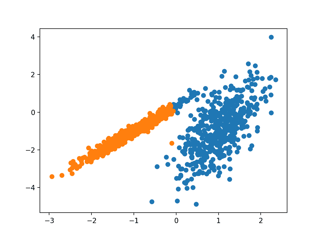
We can see that ensembles of decision trees performed the best for this problem. This suggests a few things:
- Ensembles of decision trees might be a good place to focus attention.
- Gradient boosting will likely do well if further tuned.
- A “good” performance on the problem is about 86% accuracy.
- The relatively high performance of ridge regression suggests the need for feature selection.
...
>bag: 0.862 (+/-0.034)
>rf: 0.865 (+/-0.033)
>et: 0.858 (+/-0.035)
>gbm: 0.867 (+/-0.044)
Rank=1, Name=gbm, Score=0.867 (+/- 0.044)
Rank=2, Name=rf, Score=0.865 (+/- 0.033)
Rank=3, Name=bag, Score=0.862 (+/- 0.034)
Rank=4, Name=et, Score=0.858 (+/- 0.035)
Rank=5, Name=ada, Score=0.850 (+/- 0.035)
Rank=6, Name=ridge-0.9, Score=0.848 (+/- 0.038)
Rank=7, Name=ridge-0.8, Score=0.848 (+/- 0.038)
Rank=8, Name=ridge-0.7, Score=0.848 (+/- 0.038)
Rank=9, Name=ridge-0.6, Score=0.848 (+/- 0.038)
Rank=10, Name=ridge-0.5, Score=0.848 (+/- 0.038)
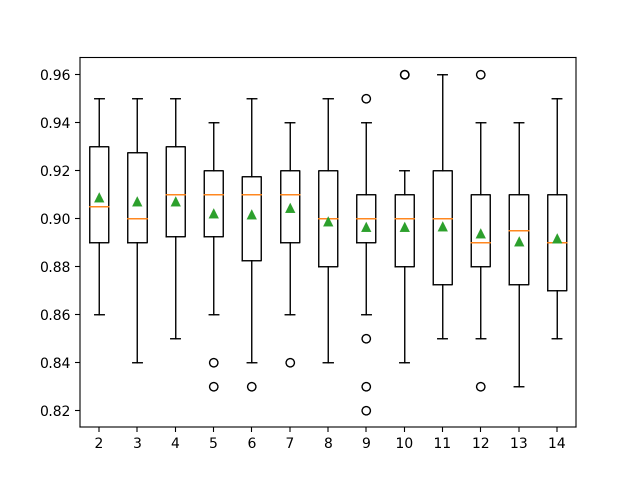
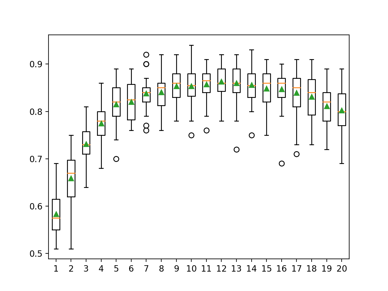
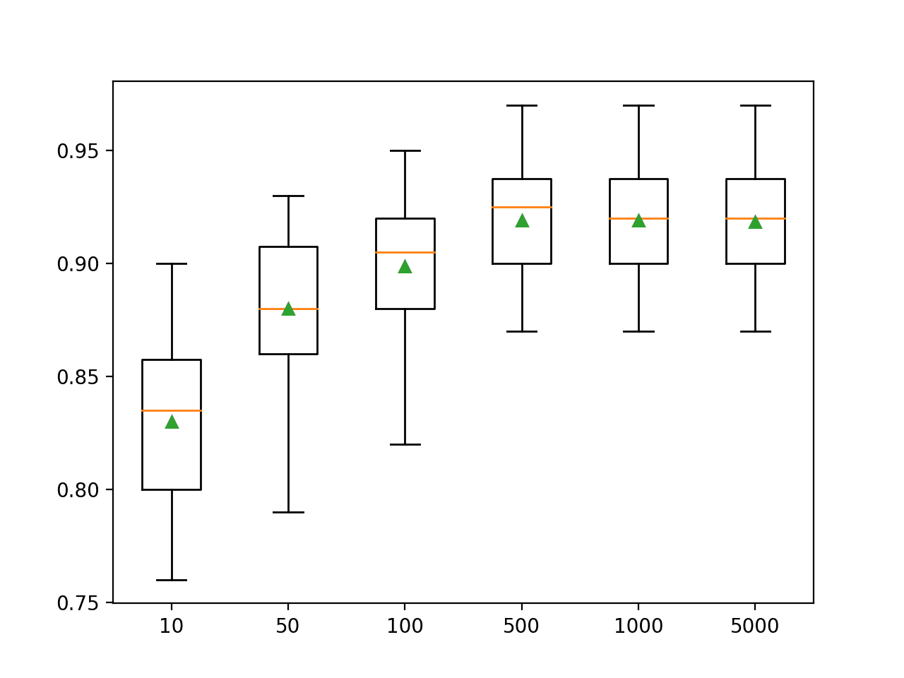
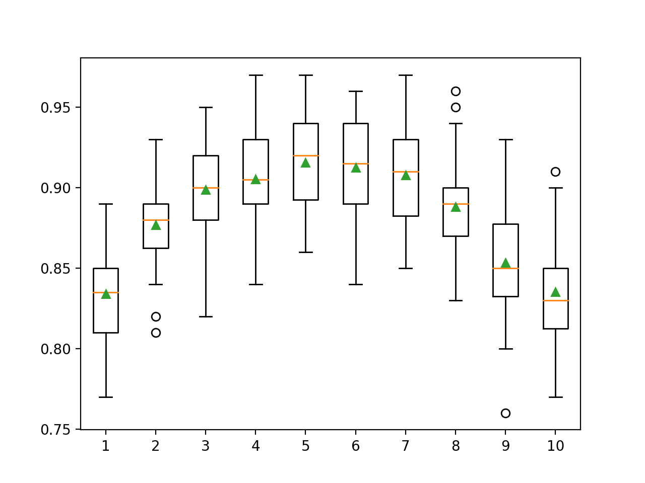
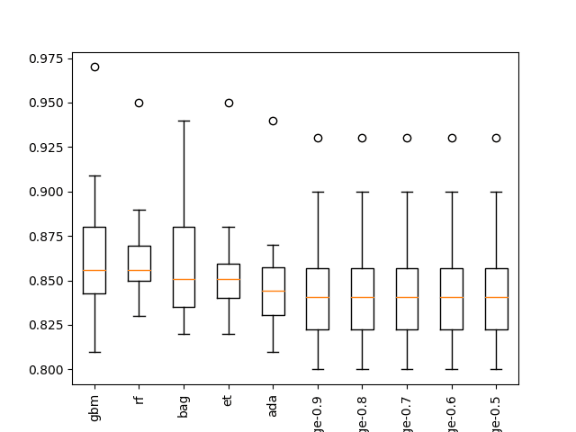
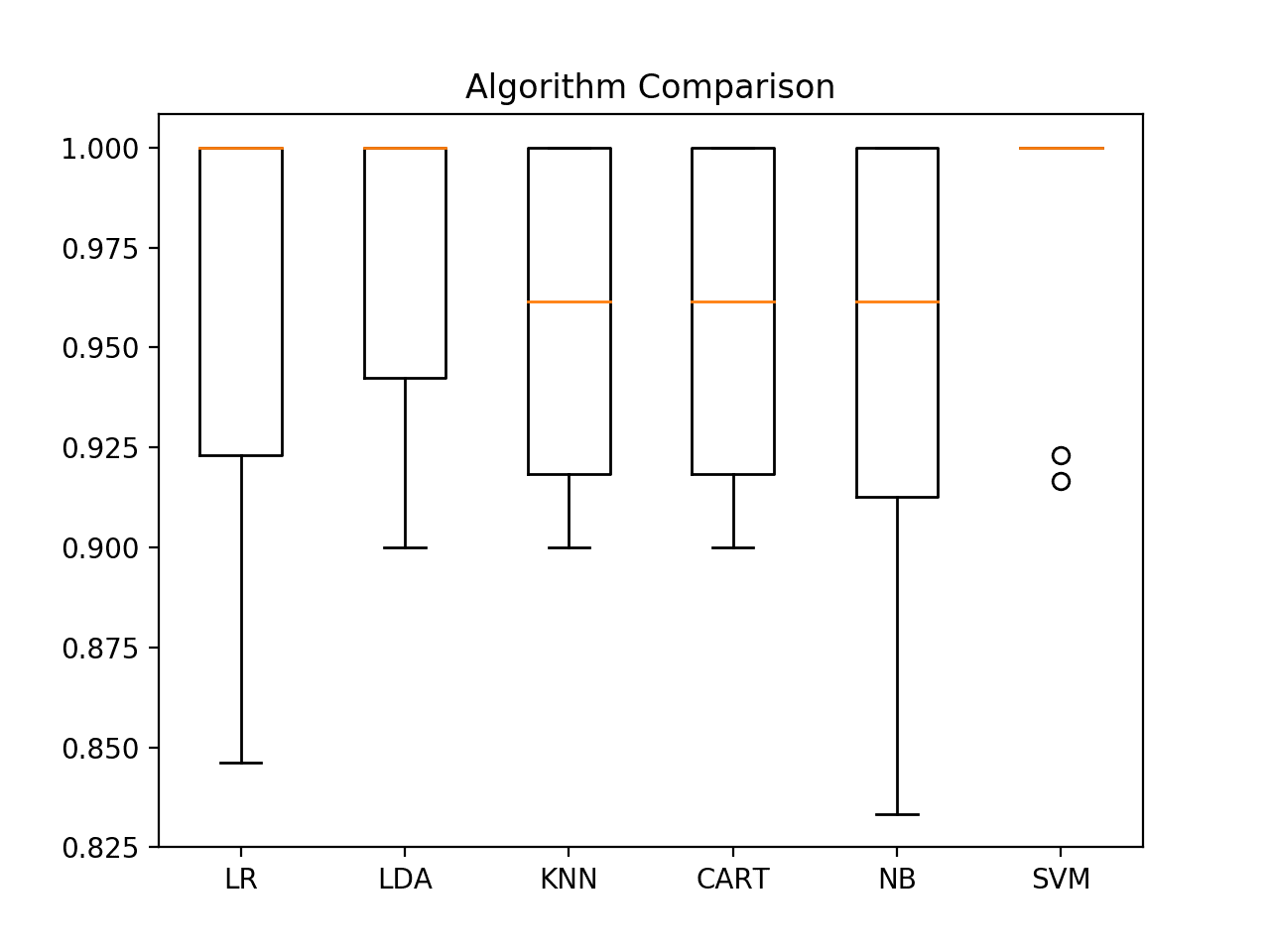
A box and whisker plot is also created to summarize the results of the top 10 well performing algorithms.
The plot shows the elevation of the methods comprised of ensembles of decision trees. The plot enforces the notion that further attention on these methods would be a good idea.
![Boxplot of top 10 Spot-Checking Algorithms on a Classification Problem]()
Boxplot of top 10 Spot-Checking Algorithms on a Classification Problem
If this were a real classification problem, I would follow-up with further spot checks, such as:
- Spot check with various different feature selection methods.
- Spot check without data scaling methods.
- Spot check with a course grid of configurations for gradient boosting in sklearn or XGBoost.
Next, we will see how we can apply the framework to a regression problem.
4. Spot-Checking for Regression
We can explore the same framework for regression predictive modeling problems with only very minor changes.
We can use the make_regression() function to generate a contrived regression problem with 1,000 examples and 50 features, some of them redundant.
The defined load_dataset() function is listed below.
# load the dataset, returns X and y elements
def load_dataset():
return make_regression(n_samples=1000, n_features=50, noise=0.1, random_state=1)
We can then specify a get_models() function that defines a suite of regression methods.
Scikit-learn does offer a wide range of linear regression methods, which is excellent. Not all of them may be required on your problem. I would recommend a minimum of linear regression and elastic net, the latter with a good suite of alpha and lambda parameters.
Nevertheless, we will test the full suite of methods on this problem, including:
Linear Algorithms
- Linear Regression
- Lasso Regression
- Ridge Regression
- Elastic Net Regression
- Huber Regression
- LARS Regression
- Lasso LARS Regression
- Passive Aggressive Regression
- RANSAC Regressor
- Stochastic Gradient Descent Regression
- Theil Regression
Nonlinear Algorithms
- k-Nearest Neighbors
- Classification and Regression Tree
- Extra Tree
- Support Vector Regression
Ensemble Algorithms
- AdaBoost
- Bagged Decision Trees
- Random Forest
- Extra Trees
- Gradient Boosting Machines
The full get_models() function is listed below.
# create a dict of standard models to evaluate {name:object}
def get_models(models=dict()):
# linear models
models['lr'] = LinearRegression()
alpha = [0.0, 0.1, 0.2, 0.3, 0.4, 0.5, 0.6, 0.7, 0.8, 0.9, 1.0]
for a in alpha:
models['lasso-'+str(a)] = Lasso(alpha=a)
for a in alpha:
models['ridge-'+str(a)] = Ridge(alpha=a)
for a1 in alpha:
for a2 in alpha:
name = 'en-' + str(a1) + '-' + str(a2)
models[name] = ElasticNet(a1, a2)
models['huber'] = HuberRegressor()
models['lars'] = Lars()
models['llars'] = LassoLars()
models['pa'] = PassiveAggressiveRegressor(max_iter=1000, tol=1e-3)
models['ranscac'] = RANSACRegressor()
models['sgd'] = SGDRegressor(max_iter=1000, tol=1e-3)
models['theil'] = TheilSenRegressor()
# non-linear models
n_neighbors = range(1, 21)
for k in n_neighbors:
models['knn-'+str(k)] = KNeighborsRegressor(n_neighbors=k)
models['cart'] = DecisionTreeRegressor()
models['extra'] = ExtraTreeRegressor()
models['svml'] = SVR(kernel='linear')
models['svmp'] = SVR(kernel='poly')
c_values = [0.1, 0.2, 0.3, 0.4, 0.5, 0.6, 0.7, 0.8, 0.9, 1.0]
for c in c_values:
models['svmr'+str(c)] = SVR(C=c)
# ensemble models
n_trees = 100
models['ada'] = AdaBoostRegressor(n_estimators=n_trees)
models['bag'] = BaggingRegressor(n_estimators=n_trees)
models['rf'] = RandomForestRegressor(n_estimators=n_trees)
models['et'] = ExtraTreesRegressor(n_estimators=n_trees)
models['gbm'] = GradientBoostingRegressor(n_estimators=n_trees)
print('Defined %d models' % len(models))
return modelsBy default, the framework uses classification accuracy as the method for evaluating model predictions.
This does not make sense for regression, and we can change this something more meaningful for regression, such as mean squared error. We can do this by passing the metric=’neg_mean_squared_error’ argument when calling evaluate_models() function.
# evaluate models
results = evaluate_models(models, metric='neg_mean_squared_error')
Note that by default scikit-learn inverts error scores so that that are maximizing instead of minimizing. This is why the mean squared error is negative and will have a negative sign when summarized. Because the score is inverted, we can continue to assume that we are maximizing scores in the summarize_results() function and do not need to specify maximize=False as we might expect when using an error metric.
The complete code example is listed below.
# regression spot check script
import warnings
from numpy import mean
from numpy import std
from matplotlib import pyplot
from sklearn.datasets import make_regression
from sklearn.model_selection import cross_val_score
from sklearn.preprocessing import StandardScaler
from sklearn.preprocessing import MinMaxScaler
from sklearn.pipeline import Pipeline
from sklearn.linear_model import LinearRegression
from sklearn.linear_model import Lasso
from sklearn.linear_model import Ridge
from sklearn.linear_model import ElasticNet
from sklearn.linear_model import HuberRegressor
from sklearn.linear_model import Lars
from sklearn.linear_model import LassoLars
from sklearn.linear_model import PassiveAggressiveRegressor
from sklearn.linear_model import RANSACRegressor
from sklearn.linear_model import SGDRegressor
from sklearn.linear_model import TheilSenRegressor
from sklearn.neighbors import KNeighborsRegressor
from sklearn.tree import DecisionTreeRegressor
from sklearn.tree import ExtraTreeRegressor
from sklearn.svm import SVR
from sklearn.ensemble import AdaBoostRegressor
from sklearn.ensemble import BaggingRegressor
from sklearn.ensemble import RandomForestRegressor
from sklearn.ensemble import ExtraTreesRegressor
from sklearn.ensemble import GradientBoostingRegressor
# load the dataset, returns X and y elements
def load_dataset():
return make_regression(n_samples=1000, n_features=50, noise=0.1, random_state=1)
# create a dict of standard models to evaluate {name:object}
def get_models(models=dict()):
# linear models
models['lr'] = LinearRegression()
alpha = [0.0, 0.1, 0.2, 0.3, 0.4, 0.5, 0.6, 0.7, 0.8, 0.9, 1.0]
for a in alpha:
models['lasso-'+str(a)] = Lasso(alpha=a)
for a in alpha:
models['ridge-'+str(a)] = Ridge(alpha=a)
for a1 in alpha:
for a2 in alpha:
name = 'en-' + str(a1) + '-' + str(a2)
models[name] = ElasticNet(a1, a2)
models['huber'] = HuberRegressor()
models['lars'] = Lars()
models['llars'] = LassoLars()
models['pa'] = PassiveAggressiveRegressor(max_iter=1000, tol=1e-3)
models['ranscac'] = RANSACRegressor()
models['sgd'] = SGDRegressor(max_iter=1000, tol=1e-3)
models['theil'] = TheilSenRegressor()
# non-linear models
n_neighbors = range(1, 21)
for k in n_neighbors:
models['knn-'+str(k)] = KNeighborsRegressor(n_neighbors=k)
models['cart'] = DecisionTreeRegressor()
models['extra'] = ExtraTreeRegressor()
models['svml'] = SVR(kernel='linear')
models['svmp'] = SVR(kernel='poly')
c_values = [0.1, 0.2, 0.3, 0.4, 0.5, 0.6, 0.7, 0.8, 0.9, 1.0]
for c in c_values:
models['svmr'+str(c)] = SVR(C=c)
# ensemble models
n_trees = 100
models['ada'] = AdaBoostRegressor(n_estimators=n_trees)
models['bag'] = BaggingRegressor(n_estimators=n_trees)
models['rf'] = RandomForestRegressor(n_estimators=n_trees)
models['et'] = ExtraTreesRegressor(n_estimators=n_trees)
models['gbm'] = GradientBoostingRegressor(n_estimators=n_trees)
print('Defined %d models' % len(models))
return models
# create a feature preparation pipeline for a model
def make_pipeline(model):
steps = list()
# standardization
steps.append(('standardize', StandardScaler()))
# normalization
steps.append(('normalize', MinMaxScaler()))
# the model
steps.append(('model', model))
# create pipeline
pipeline = Pipeline(steps=steps)
return pipeline
# evaluate a single model
def evaluate_model(X, y, model, folds, metric):
# create the pipeline
pipeline = make_pipeline(model)
# evaluate model
scores = cross_val_score(pipeline, X, y, scoring=metric, cv=folds, n_jobs=-1)
return scores
# evaluate a model and try to trap errors and and hide warnings
def robust_evaluate_model(X, y, model, folds, metric):
scores = None
try:
with warnings.catch_warnings():
warnings.filterwarnings("ignore")
scores = evaluate_model(X, y, model, folds, metric)
except:
scores = None
return scores
# evaluate a dict of models {name:object}, returns {name:score}
def evaluate_models(X, y, models, folds=10, metric='accuracy'):
results = dict()
for name, model in models.items():
# evaluate the model
scores = robust_evaluate_model(X, y, model, folds, metric)
# show process
if scores is not None:
# store a result
results[name] = scores
mean_score, std_score = mean(scores), std(scores)
print('>%s: %.3f (+/-%.3f)' % (name, mean_score, std_score))
else:
print('>%s: error' % name)
return results
# print and plot the top n results
def summarize_results(results, maximize=True, top_n=10):
# check for no results
if len(results) == 0:
print('no results')
return
# determine how many results to summarize
n = min(top_n, len(results))
# create a list of (name, mean(scores)) tuples
mean_scores = [(k,mean(v)) for k,v in results.items()]
# sort tuples by mean score
mean_scores = sorted(mean_scores, key=lambda x: x[1])
# reverse for descending order (e.g. for accuracy)
if maximize:
mean_scores = list(reversed(mean_scores))
# retrieve the top n for summarization
names = [x[0] for x in mean_scores[:n]]
scores = [results[x[0]] for x in mean_scores[:n]]
# print the top n
print()
for i in range(n):
name = names[i]
mean_score, std_score = mean(results[name]), std(results[name])
print('Rank=%d, Name=%s, Score=%.3f (+/- %.3f)' % (i+1, name, mean_score, std_score))
# boxplot for the top n
pyplot.boxplot(scores, labels=names)
_, labels = pyplot.xticks()
pyplot.setp(labels, rotation=90)
pyplot.savefig('spotcheck.png')
# load dataset
X, y = load_dataset()
# get model list
models = get_models()
# evaluate models
results = evaluate_models(X, y, models, metric='neg_mean_squared_error')
# summarize results
summarize_results(results)Running the example summarizes the performance of each model evaluated, then prints the performance of the top 10 well performing algorithms.
We can see that many of the linear algorithms perhaps found the same optimal solution on this problem. Notably those methods that performed well use regularization as a type of feature selection, allowing them to zoom in on the optimal solution.
This would suggest the importance of feature selection when modeling this problem and that linear methods would be the area to focus, at least for now.
Reviewing the printed scores of evaluated models also shows how poorly nonlinear and ensemble algorithms performed on this problem.
...
>bag: -6118.084 (+/-1558.433)
>rf: -6127.169 (+/-1594.392)
>et: -5017.062 (+/-1037.673)
>gbm: -2347.807 (+/-500.364)
Rank=1, Name=lars, Score=-0.011 (+/- 0.001)
Rank=2, Name=ranscac, Score=-0.011 (+/- 0.001)
Rank=3, Name=lr, Score=-0.011 (+/- 0.001)
Rank=4, Name=ridge-0.0, Score=-0.011 (+/- 0.001)
Rank=5, Name=en-0.0-0.1, Score=-0.011 (+/- 0.001)
Rank=6, Name=en-0.0-0.8, Score=-0.011 (+/- 0.001)
Rank=7, Name=en-0.0-0.2, Score=-0.011 (+/- 0.001)
Rank=8, Name=en-0.0-0.7, Score=-0.011 (+/- 0.001)
Rank=9, Name=en-0.0-0.0, Score=-0.011 (+/- 0.001)
Rank=10, Name=en-0.0-0.3, Score=-0.011 (+/- 0.001)
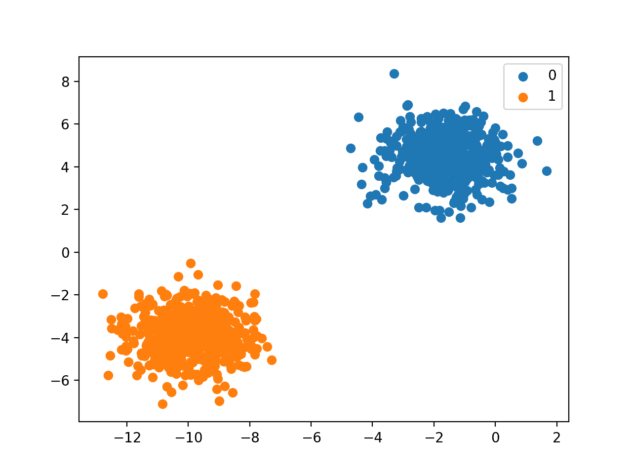
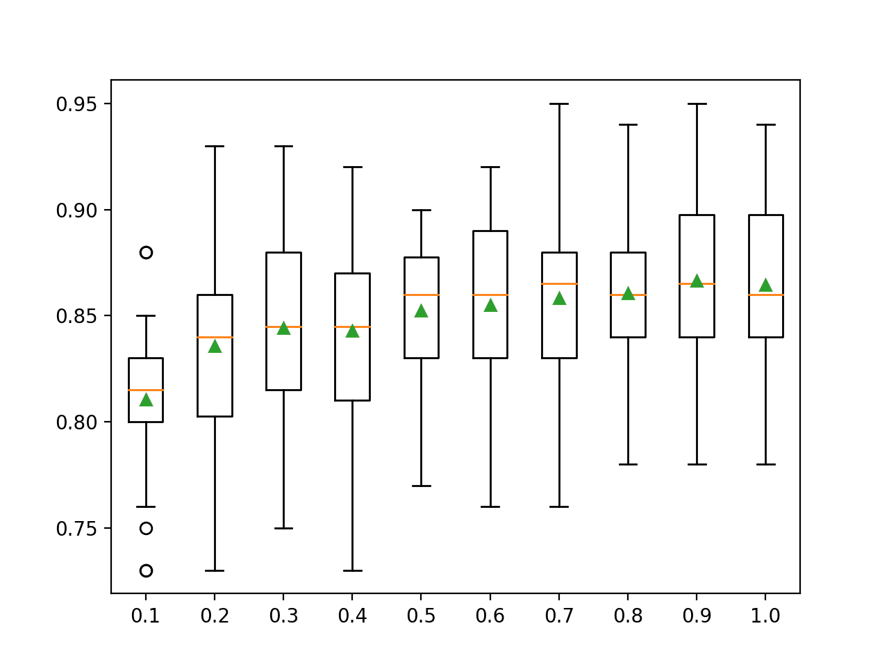
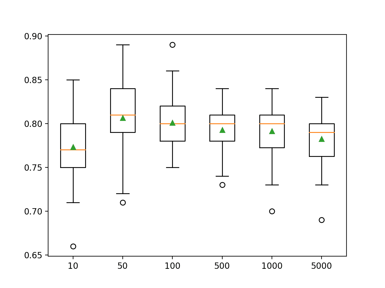
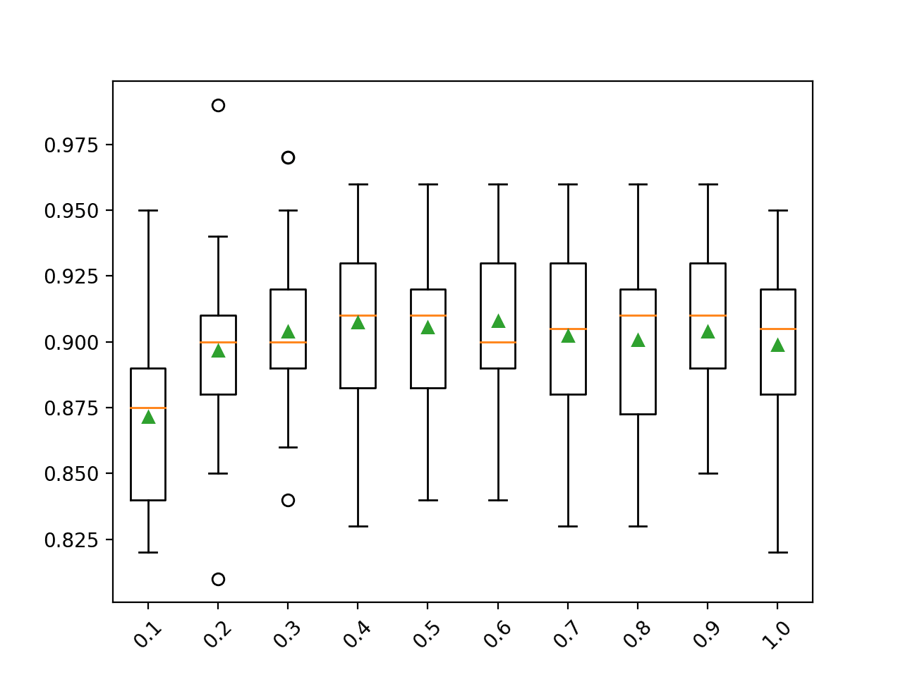
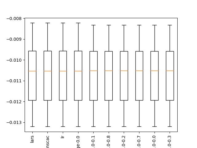
A box and whisker plot is created, not really adding value to the analysis of results in this case.
![Boxplot of top 10 Spot-Checking Algorithms on a Regression Problem]()
Boxplot of top 10 Spot-Checking Algorithms on a Regression Problem
5. Framework Extension
In this section, we explore some handy extensions of the spot check framework.
Course Grid Search for Gradient Boosting
I find myself using XGBoost and gradient boosting a lot for straight-forward classification and regression problems.
As such, I like to use a course grid across standard configuration parameters of the method when spot checking.
Below is a function to do this that can be used directly in the spot checking framework.
# define gradient boosting models
def define_gbm_models(models=dict(), use_xgb=True):
# define config ranges
rates = [0.001, 0.01, 0.1]
trees = [50, 100]
ss = [0.5, 0.7, 1.0]
depth = [3, 7, 9]
# add configurations
for l in rates:
for e in trees:
for s in ss:
for d in depth:
cfg = [l, e, s, d]
if use_xgb:
name = 'xgb-' + str(cfg)
models[name] = XGBClassifier(learning_rate=l, n_estimators=e, subsample=s, max_depth=d)
else:
name = 'gbm-' + str(cfg)
models[name] = GradientBoostingClassifier(learning_rate=l, n_estimators=e, subsample=s, max_depth=d)
print('Defined %d models' % len(models))
return modelsBy default, the function will use XGBoost models, but can use the sklearn gradient boosting model if the use_xgb argument to the function is set to False.
Again, we are not trying to optimally tune GBM on the problem, only very quickly find an area in the configuration space that may be worth investigating further.
This function can be used directly on classification and regression problems with only a minor change from “XGBClassifier” to “XGBRegressor” and “GradientBoostingClassifier” to “GradientBoostingRegressor“. For example:
# define gradient boosting models
def get_gbm_models(models=dict(), use_xgb=True):
# define config ranges
rates = [0.001, 0.01, 0.1]
trees = [50, 100]
ss = [0.5, 0.7, 1.0]
depth = [3, 7, 9]
# add configurations
for l in rates:
for e in trees:
for s in ss:
for d in depth:
cfg = [l, e, s, d]
if use_xgb:
name = 'xgb-' + str(cfg)
models[name] = XGBRegressor(learning_rate=l, n_estimators=e, subsample=s, max_depth=d)
else:
name = 'gbm-' + str(cfg)
models[name] = GradientBoostingXGBRegressor(learning_rate=l, n_estimators=e, subsample=s, max_depth=d)
print('Defined %d models' % len(models))
return modelsTo make this concrete, below is the binary classification example updated to also define XGBoost models.
# binary classification spot check script
import warnings
from numpy import mean
from numpy import std
from matplotlib import pyplot
from sklearn.datasets import make_classification
from sklearn.model_selection import cross_val_score
from sklearn.preprocessing import StandardScaler
from sklearn.preprocessing import MinMaxScaler
from sklearn.pipeline import Pipeline
from sklearn.linear_model import LogisticRegression
from sklearn.linear_model import RidgeClassifier
from sklearn.linear_model import SGDClassifier
from sklearn.linear_model import PassiveAggressiveClassifier
from sklearn.neighbors import KNeighborsClassifier
from sklearn.tree import DecisionTreeClassifier
from sklearn.tree import ExtraTreeClassifier
from sklearn.svm import SVC
from sklearn.naive_bayes import GaussianNB
from sklearn.ensemble import AdaBoostClassifier
from sklearn.ensemble import BaggingClassifier
from sklearn.ensemble import RandomForestClassifier
from sklearn.ensemble import ExtraTreesClassifier
from sklearn.ensemble import GradientBoostingClassifier
from xgboost import XGBClassifier
# load the dataset, returns X and y elements
def load_dataset():
return make_classification(n_samples=1000, n_classes=2, random_state=1)
# create a dict of standard models to evaluate {name:object}
def define_models(models=dict()):
# linear models
models['logistic'] = LogisticRegression()
alpha = [0.1, 0.2, 0.3, 0.4, 0.5, 0.6, 0.7, 0.8, 0.9, 1.0]
for a in alpha:
models['ridge-'+str(a)] = RidgeClassifier(alpha=a)
models['sgd'] = SGDClassifier(max_iter=1000, tol=1e-3)
models['pa'] = PassiveAggressiveClassifier(max_iter=1000, tol=1e-3)
# non-linear models
n_neighbors = range(1, 21)
for k in n_neighbors:
models['knn-'+str(k)] = KNeighborsClassifier(n_neighbors=k)
models['cart'] = DecisionTreeClassifier()
models['extra'] = ExtraTreeClassifier()
models['svml'] = SVC(kernel='linear')
models['svmp'] = SVC(kernel='poly')
c_values = [0.1, 0.2, 0.3, 0.4, 0.5, 0.6, 0.7, 0.8, 0.9, 1.0]
for c in c_values:
models['svmr'+str(c)] = SVC(C=c)
models['bayes'] = GaussianNB()
# ensemble models
n_trees = 100
models['ada'] = AdaBoostClassifier(n_estimators=n_trees)
models['bag'] = BaggingClassifier(n_estimators=n_trees)
models['rf'] = RandomForestClassifier(n_estimators=n_trees)
models['et'] = ExtraTreesClassifier(n_estimators=n_trees)
models['gbm'] = GradientBoostingClassifier(n_estimators=n_trees)
print('Defined %d models' % len(models))
return models
# define gradient boosting models
def define_gbm_models(models=dict(), use_xgb=True):
# define config ranges
rates = [0.001, 0.01, 0.1]
trees = [50, 100]
ss = [0.5, 0.7, 1.0]
depth = [3, 7, 9]
# add configurations
for l in rates:
for e in trees:
for s in ss:
for d in depth:
cfg = [l, e, s, d]
if use_xgb:
name = 'xgb-' + str(cfg)
models[name] = XGBClassifier(learning_rate=l, n_estimators=e, subsample=s, max_depth=d)
else:
name = 'gbm-' + str(cfg)
models[name] = GradientBoostingClassifier(learning_rate=l, n_estimators=e, subsample=s, max_depth=d)
print('Defined %d models' % len(models))
return models
# create a feature preparation pipeline for a model
def make_pipeline(model):
steps = list()
# standardization
steps.append(('standardize', StandardScaler()))
# normalization
steps.append(('normalize', MinMaxScaler()))
# the model
steps.append(('model', model))
# create pipeline
pipeline = Pipeline(steps=steps)
return pipeline
# evaluate a single model
def evaluate_model(X, y, model, folds, metric):
# create the pipeline
pipeline = make_pipeline(model)
# evaluate model
scores = cross_val_score(pipeline, X, y, scoring=metric, cv=folds, n_jobs=-1)
return scores
# evaluate a model and try to trap errors and and hide warnings
def robust_evaluate_model(X, y, model, folds, metric):
scores = None
try:
with warnings.catch_warnings():
warnings.filterwarnings("ignore")
scores = evaluate_model(X, y, model, folds, metric)
except:
scores = None
return scores
# evaluate a dict of models {name:object}, returns {name:score}
def evaluate_models(X, y, models, folds=10, metric='accuracy'):
results = dict()
for name, model in models.items():
# evaluate the model
scores = robust_evaluate_model(X, y, model, folds, metric)
# show process
if scores is not None:
# store a result
results[name] = scores
mean_score, std_score = mean(scores), std(scores)
print('>%s: %.3f (+/-%.3f)' % (name, mean_score, std_score))
else:
print('>%s: error' % name)
return results
# print and plot the top n results
def summarize_results(results, maximize=True, top_n=10):
# check for no results
if len(results) == 0:
print('no results')
return
# determine how many results to summarize
n = min(top_n, len(results))
# create a list of (name, mean(scores)) tuples
mean_scores = [(k,mean(v)) for k,v in results.items()]
# sort tuples by mean score
mean_scores = sorted(mean_scores, key=lambda x: x[1])
# reverse for descending order (e.g. for accuracy)
if maximize:
mean_scores = list(reversed(mean_scores))
# retrieve the top n for summarization
names = [x[0] for x in mean_scores[:n]]
scores = [results[x[0]] for x in mean_scores[:n]]
# print the top n
print()
for i in range(n):
name = names[i]
mean_score, std_score = mean(results[name]), std(results[name])
print('Rank=%d, Name=%s, Score=%.3f (+/- %.3f)' % (i+1, name, mean_score, std_score))
# boxplot for the top n
pyplot.boxplot(scores, labels=names)
_, labels = pyplot.xticks()
pyplot.setp(labels, rotation=90)
pyplot.savefig('spotcheck.png')
# load dataset
X, y = load_dataset()
# get model list
models = define_models()
# add gbm models
models = define_gbm_models(models)
# evaluate models
results = evaluate_models(X, y, models)
# summarize results
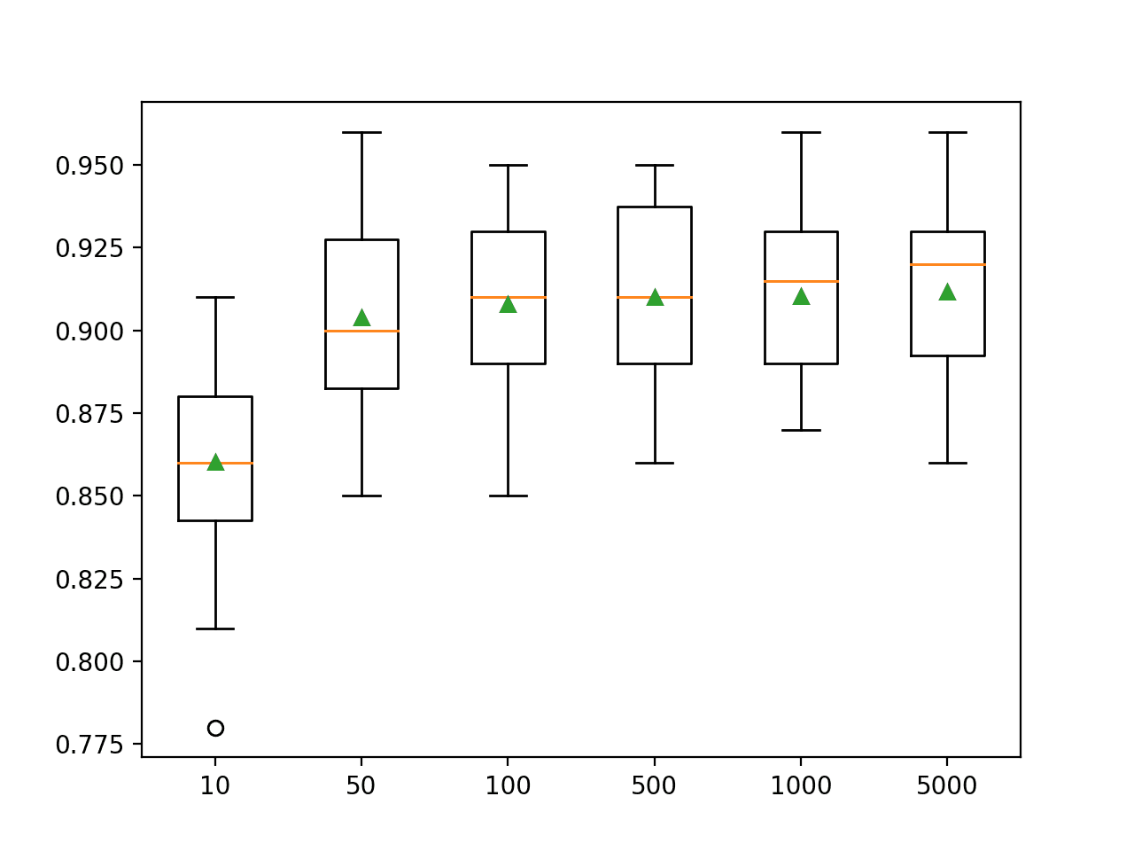
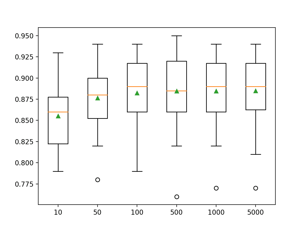
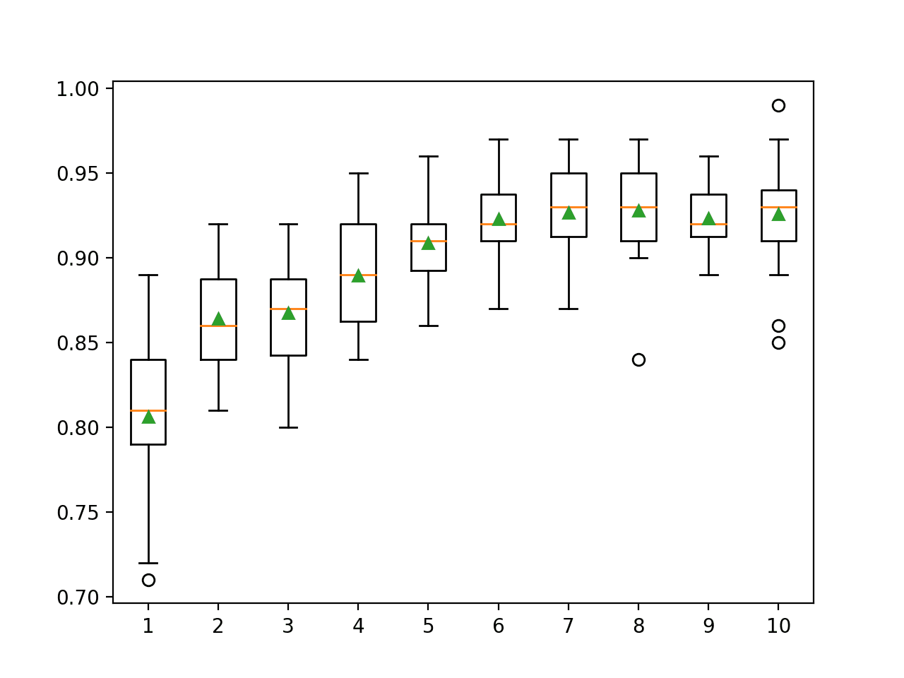
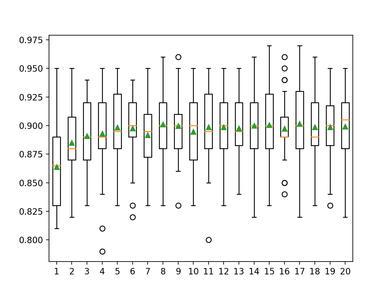
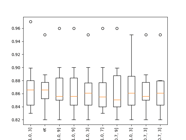
summarize_results(results)Running the example shows that indeed some XGBoost models perform well on the problem.
...
>xgb-[0.1, 100, 1.0, 3]: 0.864 (+/-0.044)
>xgb-[0.1, 100, 1.0, 7]: 0.865 (+/-0.036)
>xgb-[0.1, 100, 1.0, 9]: 0.867 (+/-0.039)
Rank=1, Name=xgb-[0.1, 50, 1.0, 3], Score=0.872 (+/- 0.039)
Rank=2, Name=et, Score=0.869 (+/- 0.033)
Rank=3, Name=xgb-[0.1, 50, 1.0, 9], Score=0.868 (+/- 0.038)
Rank=4, Name=xgb-[0.1, 100, 1.0, 9], Score=0.867 (+/- 0.039)
Rank=5, Name=xgb-[0.01, 50, 1.0, 3], Score=0.867 (+/- 0.035)
Rank=6, Name=xgb-[0.1, 50, 1.0, 7], Score=0.867 (+/- 0.037)
Rank=7, Name=xgb-[0.001, 100, 0.7, 9], Score=0.866 (+/- 0.040)
Rank=8, Name=xgb-[0.01, 100, 1.0, 3], Score=0.866 (+/- 0.037)
Rank=9, Name=xgb-[0.001, 100, 0.7, 3], Score=0.866 (+/- 0.034)
Rank=10, Name=xgb-[0.01, 50, 0.7, 3], Score=0.866 (+/- 0.034)
![Boxplot of top 10 Spot-Checking Algorithms on a Classification Problem with XGBoost]()
Boxplot of top 10 Spot-Checking Algorithms on a Classification Problem with XGBoost
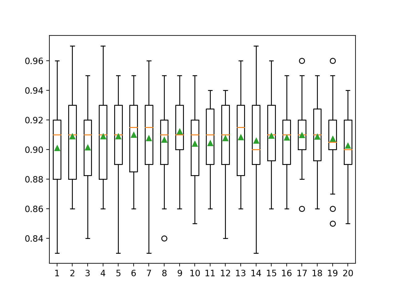
Repeated Evaluations
The above results also highlight the noisy nature of the evaluations, e.g. the results of extra trees in this run are different from the run above (0.858 vs 0.869).
We are using k-fold cross-validation to produce a population of scores, but the population is small and the calculated mean will be noisy.
This is fine as long as we take the spot-check results as a starting point and not definitive results of an algorithm on the problem. This is hard to do; it takes discipline in the practitioner.
Alternately, you may want to adapt the framework such that the model evaluation scheme better matches the model evaluation scheme you intend to use for your specific problem.
For example, when evaluating stochastic algorithms like bagged or boosted decision trees, it is a good idea to run each experiment multiple times on the same train/test sets (called repeats) in order to account for the stochastic nature of the learning algorithm.
We can update the evaluate_model() function to repeat the evaluation of a given model n-times, with a different split of the data each time, then return all scores. For example, three repeats of 10-fold cross-validation will result in 30 scores from each to calculate a mean performance of a model.
# evaluate a single model
def evaluate_model(X, y, model, folds, repeats, metric):
# create the pipeline
pipeline = make_pipeline(model)
# evaluate model
scores = list()
# repeat model evaluation n times
for _ in range(repeats):
# perform run
scores_r = cross_val_score(pipeline, X, y, scoring=metric, cv=folds, n_jobs=-1)
# add scores to list
scores += scores_r.tolist()
return scores
Alternately, you may prefer to calculate a mean score from each k-fold cross-validation run, then calculate a grand mean of all runs, as described in:
We can then update the robust_evaluate_model() function to pass down the repeats argument and the evaluate_models() function to define a default, such as 3.
A complete example of the binary classification example with three repeats of model evaluation is listed below.
# binary classification spot check script
import warnings
from numpy import mean
from numpy import std
from matplotlib import pyplot
from sklearn.datasets import make_classification
from sklearn.model_selection import cross_val_score
from sklearn.preprocessing import StandardScaler
from sklearn.preprocessing import MinMaxScaler
from sklearn.pipeline import Pipeline
from sklearn.linear_model import LogisticRegression
from sklearn.linear_model import RidgeClassifier
from sklearn.linear_model import SGDClassifier
from sklearn.linear_model import PassiveAggressiveClassifier
from sklearn.neighbors import KNeighborsClassifier
from sklearn.tree import DecisionTreeClassifier
from sklearn.tree import ExtraTreeClassifier
from sklearn.svm import SVC
from sklearn.naive_bayes import GaussianNB
from sklearn.ensemble import AdaBoostClassifier
from sklearn.ensemble import BaggingClassifier
from sklearn.ensemble import RandomForestClassifier
from sklearn.ensemble import ExtraTreesClassifier
from sklearn.ensemble import GradientBoostingClassifier
# load the dataset, returns X and y elements
def load_dataset():
return make_classification(n_samples=1000, n_classes=2, random_state=1)
# create a dict of standard models to evaluate {name:object}
def define_models(models=dict()):
# linear models
models['logistic'] = LogisticRegression()
alpha = [0.1, 0.2, 0.3, 0.4, 0.5, 0.6, 0.7, 0.8, 0.9, 1.0]
for a in alpha:
models['ridge-'+str(a)] = RidgeClassifier(alpha=a)
models['sgd'] = SGDClassifier(max_iter=1000, tol=1e-3)
models['pa'] = PassiveAggressiveClassifier(max_iter=1000, tol=1e-3)
# non-linear models
n_neighbors = range(1, 21)
for k in n_neighbors:
models['knn-'+str(k)] = KNeighborsClassifier(n_neighbors=k)
models['cart'] = DecisionTreeClassifier()
models['extra'] = ExtraTreeClassifier()
models['svml'] = SVC(kernel='linear')
models['svmp'] = SVC(kernel='poly')
c_values = [0.1, 0.2, 0.3, 0.4, 0.5, 0.6, 0.7, 0.8, 0.9, 1.0]
for c in c_values:
models['svmr'+str(c)] = SVC(C=c)
models['bayes'] = GaussianNB()
# ensemble models
n_trees = 100
models['ada'] = AdaBoostClassifier(n_estimators=n_trees)
models['bag'] = BaggingClassifier(n_estimators=n_trees)
models['rf'] = RandomForestClassifier(n_estimators=n_trees)
models['et'] = ExtraTreesClassifier(n_estimators=n_trees)
models['gbm'] = GradientBoostingClassifier(n_estimators=n_trees)
print('Defined %d models' % len(models))
return models
# create a feature preparation pipeline for a model
def make_pipeline(model):
steps = list()
# standardization
steps.append(('standardize', StandardScaler()))
# normalization
steps.append(('normalize', MinMaxScaler()))
# the model
steps.append(('model', model))
# create pipeline
pipeline = Pipeline(steps=steps)
return pipeline
# evaluate a single model
def evaluate_model(X, y, model, folds, repeats, metric):
# create the pipeline
pipeline = make_pipeline(model)
# evaluate model
scores = list()
# repeat model evaluation n times
for _ in range(repeats):
# perform run
scores_r = cross_val_score(pipeline, X, y, scoring=metric, cv=folds, n_jobs=-1)
# add scores to list
scores += scores_r.tolist()
return scores
# evaluate a model and try to trap errors and hide warnings
def robust_evaluate_model(X, y, model, folds, repeats, metric):
scores = None
try:
with warnings.catch_warnings():
warnings.filterwarnings("ignore")
scores = evaluate_model(X, y, model, folds, repeats, metric)
except:
scores = None
return scores
# evaluate a dict of models {name:object}, returns {name:score}
def evaluate_models(X, y, models, folds=10, repeats=3, metric='accuracy'):
results = dict()
for name, model in models.items():
# evaluate the model
scores = robust_evaluate_model(X, y, model, folds, repeats, metric)
# show process
if scores is not None:
# store a result
results[name] = scores
mean_score, std_score = mean(scores), std(scores)
print('>%s: %.3f (+/-%.3f)' % (name, mean_score, std_score))
else:
print('>%s: error' % name)
return results
# print and plot the top n results
def summarize_results(results, maximize=True, top_n=10):
# check for no results
if len(results) == 0:
print('no results')
return
# determine how many results to summarize
n = min(top_n, len(results))
# create a list of (name, mean(scores)) tuples
mean_scores = [(k,mean(v)) for k,v in results.items()]
# sort tuples by mean score
mean_scores = sorted(mean_scores, key=lambda x: x[1])
# reverse for descending order (e.g. for accuracy)
if maximize:
mean_scores = list(reversed(mean_scores))
# retrieve the top n for summarization
names = [x[0] for x in mean_scores[:n]]
scores = [results[x[0]] for x in mean_scores[:n]]
# print the top n
print()
for i in range(n):
name = names[i]
mean_score, std_score = mean(results[name]), std(results[name])
print('Rank=%d, Name=%s, Score=%.3f (+/- %.3f)' % (i+1, name, mean_score, std_score))
# boxplot for the top n
pyplot.boxplot(scores, labels=names)
_, labels = pyplot.xticks()
pyplot.setp(labels, rotation=90)
pyplot.savefig('spotcheck.png')
# load dataset
X, y = load_dataset()
# get model list
models = define_models()
# evaluate models
results = evaluate_models(X, y, models)
# summarize results
summarize_results(results)Running the example produces a more robust estimate of the scores.
...
>bag: 0.861 (+/-0.037)
>rf: 0.859 (+/-0.036)
>et: 0.869 (+/-0.035)
>gbm: 0.867 (+/-0.044)
Rank=1, Name=et, Score=0.869 (+/- 0.035)
Rank=2, Name=gbm, Score=0.867 (+/- 0.044)
Rank=3, Name=bag, Score=0.861 (+/- 0.037)
Rank=4, Name=rf, Score=0.859 (+/- 0.036)
Rank=5, Name=ada, Score=0.850 (+/- 0.035)
Rank=6, Name=ridge-0.9, Score=0.848 (+/- 0.038)
Rank=7, Name=ridge-0.8, Score=0.848 (+/- 0.038)
Rank=8, Name=ridge-0.7, Score=0.848 (+/- 0.038)
Rank=9, Name=ridge-0.6, Score=0.848 (+/- 0.038)
Rank=10, Name=ridge-0.5, Score=0.848 (+/- 0.038)
There will still be some variance in the reported means, but less than a single run of k-fold cross-validation.
The number of repeats may be increased to further reduce this variance, at the cost of longer run times, and perhaps against the intent of spot checking.
Varied Input Representations
I am a big fan of avoiding assumptions and recommendations for data representations prior to fitting models.
Instead, I like to also spot-check multiple representations and transforms of input data, which I refer to as views. I explain this more in the post:
We can update the framework to spot-check multiple different representations for each model.
One way to do this is to update the evaluate_models() function so that we can provide a list of make_pipeline() functions that can be used for each defined model.
# evaluate a dict of models {name:object}, returns {name:score}
def evaluate_models(X, y, models, pipe_funcs, folds=10, metric='accuracy'):
results = dict()
for name, model in models.items():
# evaluate model under each preparation function
for i in range(len(pipe_funcs)):
# evaluate the model
scores = robust_evaluate_model(X, y, model, folds, metric, pipe_funcs[i])
# update name
run_name = str(i) + name
# show process
if scores is not None:
# store a result
results[run_name] = scores
mean_score, std_score = mean(scores), std(scores)
print('>%s: %.3f (+/-%.3f)' % (run_name, mean_score, std_score))
else:
print('>%s: error' % run_name)
return resultsThe chosen pipeline function can then be passed along down to the robust_evaluate_model() function and to the evaluate_model() function where it can be used.
We can then define a bunch of different pipeline functions; for example:
# no transforms pipeline
def pipeline_none(model):
return model
# standardize transform pipeline
def pipeline_standardize(model):
steps = list()
# standardization
steps.append(('standardize', StandardScaler()))
# the model
steps.append(('model', model))
# create pipeline
pipeline = Pipeline(steps=steps)
return pipeline
# normalize transform pipeline
def pipeline_normalize(model):
steps = list()
# normalization
steps.append(('normalize', MinMaxScaler()))
# the model
steps.append(('model', model))
# create pipeline
pipeline = Pipeline(steps=steps)
return pipeline
# standardize and normalize pipeline
def pipeline_std_norm(model):
steps = list()
# standardization
steps.append(('standardize', StandardScaler()))
# normalization
steps.append(('normalize', MinMaxScaler()))
# the model
steps.append(('model', model))
# create pipeline
pipeline = Pipeline(steps=steps)
return pipelineThen create a list of these function names that can be provided to the evaluate_models() function.
# define transform pipelines
pipelines = [pipeline_none, pipeline_standardize, pipeline_normalize, pipeline_std_norm]
The complete example of the classification case updated to spot check pipeline transforms is listed below.
# binary classification spot check script
import warnings
from numpy import mean
from numpy import std
from matplotlib import pyplot
from sklearn.datasets import make_classification
from sklearn.model_selection import cross_val_score
from sklearn.preprocessing import StandardScaler
from sklearn.preprocessing import MinMaxScaler
from sklearn.pipeline import Pipeline
from sklearn.linear_model import LogisticRegression
from sklearn.linear_model import RidgeClassifier
from sklearn.linear_model import SGDClassifier
from sklearn.linear_model import PassiveAggressiveClassifier
from sklearn.neighbors import KNeighborsClassifier
from sklearn.tree import DecisionTreeClassifier
from sklearn.tree import ExtraTreeClassifier
from sklearn.svm import SVC
from sklearn.naive_bayes import GaussianNB
from sklearn.ensemble import AdaBoostClassifier
from sklearn.ensemble import BaggingClassifier
from sklearn.ensemble import RandomForestClassifier
from sklearn.ensemble import ExtraTreesClassifier
from sklearn.ensemble import GradientBoostingClassifier
# load the dataset, returns X and y elements
def load_dataset():
return make_classification(n_samples=1000, n_classes=2, random_state=1)
# create a dict of standard models to evaluate {name:object}
def define_models(models=dict()):
# linear models
models['logistic'] = LogisticRegression()
alpha = [0.1, 0.2, 0.3, 0.4, 0.5, 0.6, 0.7, 0.8, 0.9, 1.0]
for a in alpha:
models['ridge-'+str(a)] = RidgeClassifier(alpha=a)
models['sgd'] = SGDClassifier(max_iter=1000, tol=1e-3)
models['pa'] = PassiveAggressiveClassifier(max_iter=1000, tol=1e-3)
# non-linear models
n_neighbors = range(1, 21)
for k in n_neighbors:
models['knn-'+str(k)] = KNeighborsClassifier(n_neighbors=k)
models['cart'] = DecisionTreeClassifier()
models['extra'] = ExtraTreeClassifier()
models['svml'] = SVC(kernel='linear')
models['svmp'] = SVC(kernel='poly')
c_values = [0.1, 0.2, 0.3, 0.4, 0.5, 0.6, 0.7, 0.8, 0.9, 1.0]
for c in c_values:
models['svmr'+str(c)] = SVC(C=c)
models['bayes'] = GaussianNB()
# ensemble models
n_trees = 100
models['ada'] = AdaBoostClassifier(n_estimators=n_trees)
models['bag'] = BaggingClassifier(n_estimators=n_trees)
models['rf'] = RandomForestClassifier(n_estimators=n_trees)
models['et'] = ExtraTreesClassifier(n_estimators=n_trees)
models['gbm'] = GradientBoostingClassifier(n_estimators=n_trees)
print('Defined %d models' % len(models))
return models
# no transforms pipeline
def pipeline_none(model):
return model
# standardize transform pipeline
def pipeline_standardize(model):
steps = list()
# standardization
steps.append(('standardize', StandardScaler()))
# the model
steps.append(('model', model))
# create pipeline
pipeline = Pipeline(steps=steps)
return pipeline
# normalize transform pipeline
def pipeline_normalize(model):
steps = list()
# normalization
steps.append(('normalize', MinMaxScaler()))
# the model
steps.append(('model', model))
# create pipeline
pipeline = Pipeline(steps=steps)
return pipeline
# standardize and normalize pipeline
def pipeline_std_norm(model):
steps = list()
# standardization
steps.append(('standardize', StandardScaler()))
# normalization
steps.append(('normalize', MinMaxScaler()))
# the model
steps.append(('model', model))
# create pipeline
pipeline = Pipeline(steps=steps)
return pipeline
# evaluate a single model
def evaluate_model(X, y, model, folds, metric, pipe_func):
# create the pipeline
pipeline = pipe_func(model)
# evaluate model
scores = cross_val_score(pipeline, X, y, scoring=metric, cv=folds, n_jobs=-1)
return scores
# evaluate a model and try to trap errors and and hide warnings
def robust_evaluate_model(X, y, model, folds, metric, pipe_func):
scores = None
try:
with warnings.catch_warnings():
warnings.filterwarnings("ignore")
scores = evaluate_model(X, y, model, folds, metric, pipe_func)
except:
scores = None
return scores
# evaluate a dict of models {name:object}, returns {name:score}
def evaluate_models(X, y, models, pipe_funcs, folds=10, metric='accuracy'):
results = dict()
for name, model in models.items():
# evaluate model under each preparation function
for i in range(len(pipe_funcs)):
# evaluate the model
scores = robust_evaluate_model(X, y, model, folds, metric, pipe_funcs[i])
# update name
run_name = str(i) + name
# show process
if scores is not None:
# store a result
results[run_name] = scores
mean_score, std_score = mean(scores), std(scores)
print('>%s: %.3f (+/-%.3f)' % (run_name, mean_score, std_score))
else:
print('>%s: error' % run_name)
return results
# print and plot the top n results
def summarize_results(results, maximize=True, top_n=10):
# check for no results
if len(results) == 0:
print('no results')
return
# determine how many results to summarize
n = min(top_n, len(results))
# create a list of (name, mean(scores)) tuples
mean_scores = [(k,mean(v)) for k,v in results.items()]
# sort tuples by mean score
mean_scores = sorted(mean_scores, key=lambda x: x[1])
# reverse for descending order (e.g. for accuracy)
if maximize:
mean_scores = list(reversed(mean_scores))
# retrieve the top n for summarization
names = [x[0] for x in mean_scores[:n]]
scores = [results[x[0]] for x in mean_scores[:n]]
# print the top n
print()
for i in range(n):
name = names[i]
mean_score, std_score = mean(results[name]), std(results[name])
print('Rank=%d, Name=%s, Score=%.3f (+/- %.3f)' % (i+1, name, mean_score, std_score))
# boxplot for the top n
pyplot.boxplot(scores, labels=names)
_, labels = pyplot.xticks()
pyplot.setp(labels, rotation=90)
pyplot.savefig('spotcheck.png')
# load dataset
X, y = load_dataset()
# get model list
models = define_models()
# define transform pipelines
pipelines = [pipeline_none, pipeline_standardize, pipeline_normalize, pipeline_std_norm]
# evaluate models
results = evaluate_models(X, y, models, pipelines)
# summarize results
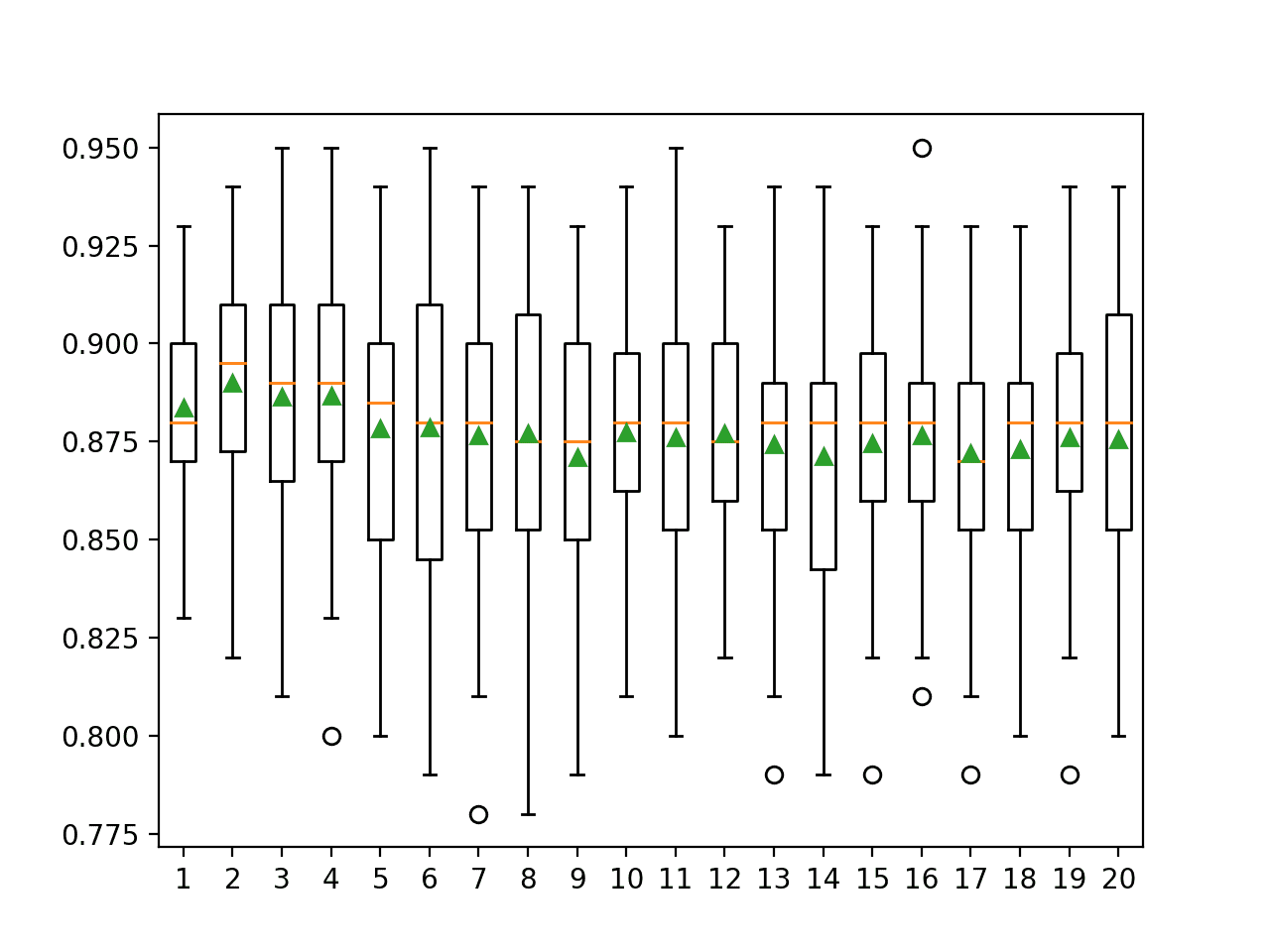
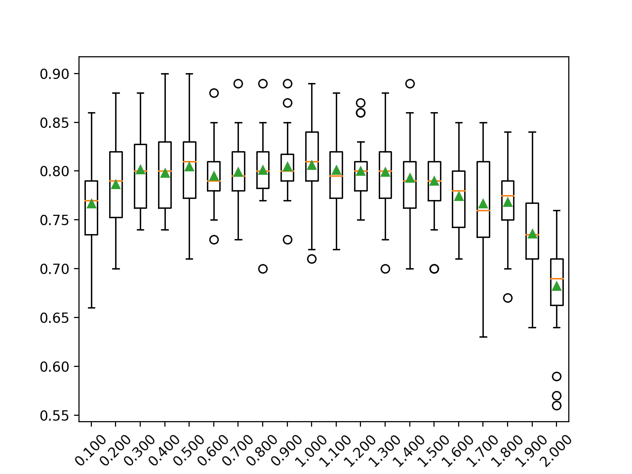
summarize_results(results)Running the example shows that we differentiate the results for each pipeline by adding the pipeline number to the beginning of the algorithm description name, e.g. ‘0rf‘ means RF with the first pipeline, which is no transforms.
The ensembles of trees algorithms perform well on this problem, and these algorithms are invariant to data scaling. This means that their results on each pipeline will be similar (or the same) and in turn they will crowd out other algorithms in the top-10 list.
...
>0gbm: 0.865 (+/-0.044)
>1gbm: 0.865 (+/-0.044)
>2gbm: 0.865 (+/-0.044)
>3gbm: 0.865 (+/-0.044)
Rank=1, Name=3rf, Score=0.870 (+/- 0.034)
Rank=2, Name=2rf, Score=0.870 (+/- 0.034)
Rank=3, Name=1rf, Score=0.870 (+/- 0.034)
Rank=4, Name=0rf, Score=0.870 (+/- 0.034)
Rank=5, Name=3bag, Score=0.866 (+/- 0.039)
Rank=6, Name=2bag, Score=0.866 (+/- 0.039)
Rank=7, Name=1bag, Score=0.866 (+/- 0.039)
Rank=8, Name=0bag, Score=0.866 (+/- 0.039)
Rank=9, Name=3gbm, Score=0.865 (+/- 0.044)
Rank=10, Name=2gbm, Score=0.865 (+/- 0.044)
Further Reading
This section provides more resources on the topic if you are looking to go deeper.
Summary
In this tutorial, you discovered the usefulness of spot-checking algorithms on a new predictive modeling problem and how to develop a standard framework for spot-checking algorithms in python for classification and regression problems.
Specifically, you learned:
- Spot-checking provides a way to quickly discover the types of algorithms that perform well on your predictive modeling problem.
- How to develop a generic framework for loading data, defining models, evaluating models, and summarizing results.
- How to apply the framework for classification and regression problems.
Have you used this framework or do you have some further suggestions to improve it?
Let me know in the comments.
Do you have any questions?
Ask your questions in the comments below and I will do my best to answer.
The post How to Develop a Framework to Spot-Check Machine Learning Algorithms in Python appeared first on Machine Learning Mastery.