Quantcast
Channel: MachineLearningMastery.com
Viewing all 263 articles
Browse latest View live

Radius Neighbors Classifier Algorithm With Python

$
0
0

Radius Neighbors Classifier is a classification machine learning algorithm.

It is an extension to the k-nearest neighbors algorithm that makes predictions using all examples in the radius of a new example rather than the k-closest neighbors.

As such, the radius-based approach to selecting neighbors is more appropriate for sparse data, preventing examples that are far away in the feature space from contributing to a prediction.

In this tutorial, you will discover the Radius Neighbors Classifier classification machine learning algorithm.

After completing this tutorial, you will know:

  • The Nearest Radius Neighbors Classifier is a simple extension of the k-nearest neighbors classification algorithm.
  • How to fit, evaluate, and make predictions with the Radius Neighbors Classifier model with Scikit-Learn.
  • How to tune the hyperparameters of the Radius Neighbors Classifier algorithm on a given dataset.

Let’s get started.

Radius Neighbors Classifier Algorithm With Python

Radius Neighbors Classifier Algorithm With Python
Photo by J. Triepke, some rights reserved.

Tutorial Overview

This tutorial is divided into three parts; they are:

  1. Radius Neighbors Classifier
  2. Radius Neighbors Classifier With Scikit-Learn
  3. Tune Radius Neighbors Classifier Hyperparameters

Radius Neighbors Classifier

Radius Neighbors is a classification machine learning algorithm.

It is based on the k-nearest neighbors algorithm, or kNN. kNN involves taking the entire training dataset and storing it. Then, at prediction time, the k-closest examples in the training dataset are located for each new example for which we want to predict. The mode (most common value) class label from the k neighbors is then assigned to the new example.

For more on the k-nearest neighbours algorithm, see the tutorial:

The Radius Neighbors Classifier is similar in that training involves storing the entire training dataset. The way that the training dataset is used during prediction is different.

Instead of locating the k-neighbors, the Radius Neighbors Classifier locates all examples in the training dataset that are within a given radius of the new example. The radius neighbors are then used to make a prediction for the new example.

The radius is defined in the feature space and generally assumes that the input variables are numeric and scaled to the range 0-1, e.g. normalized.

The radius-based approach to locating neighbors is appropriate for those datasets where it is desirable for the contribution of neighbors to be proportional to the density of examples in the feature space.

Given a fixed radius, dense regions of the feature space will contribute more information and sparse regions will contribute less information. It is this latter case that is most desirable and it prevents examples very far in feature space from the new example from contributing to the prediction.

As such, the Radius Neighbors Classifier may be more appropriate for prediction problems where there are sparse regions of the feature space.

Given that the radius is fixed in all dimensions of the feature space, it will become less effective as the number of input features is increased, which causes examples in the feature space to spread further and further apart. This property is referred to as the curse of dimensionality.

Radius Neighbors Classifier With Scikit-Learn

The Radius Neighbors Classifier is available in the scikit-learn Python machine learning library via the RadiusNeighborsClassifier class.

The class allows you to specify the size of the radius used when making a prediction via the “radius” argument, which defaults to 1.0.

...
# create the model
model = RadiusNeighborsClassifier(radius=1.0)

Another important hyperparameter is the “weights” argument that controls whether neighbors contribute to the prediction in a ‘uniform‘ manner or inverse to the distance (‘distance‘) from the example. Uniform weight is used by default.

...
# create the model
model = RadiusNeighborsClassifier(weights='uniform')

We can demonstrate the Radius Neighbors Classifier with a worked example.

First, let’s define a synthetic classification dataset.

We will use the make_classification() function to create a dataset with 1,000 examples, each with 20 input variables.

The example below creates and summarizes the dataset.

# test classification dataset
from sklearn.datasets import make_classification
# define dataset
X, y = make_classification(n_samples=1000, n_features=20, n_informative=15, n_redundant=5, random_state=1)
# summarize the dataset
print(X.shape, y.shape)

Running the example creates the dataset and confirms the number of rows and columns of the dataset.

(1000, 20) (1000,)

We can fit and evaluate a Radius Neighbors Classifier model using repeated stratified k-fold cross-validation via the RepeatedStratifiedKFold class. We will use 10 folds and three repeats in the test harness.

We will use the default configuration.

...
# create the model
model = RadiusNeighborsClassifier()

It is important that the feature space is scaled prior to preparing and using the model.

We can achieve this by using the MinMaxScaler to normalize the input features and use a Pipeline to first apply the scaling, then use the model.

...
# define model
model = RadiusNeighborsClassifier()
# create pipeline
pipeline = Pipeline(steps=[('norm', MinMaxScaler()),('model',model)])

The complete example of evaluating the Radius Neighbors Classifier model for the synthetic binary classification task is listed below.

# evaluate an radius neighbors classifier model on the dataset
from numpy import mean
from numpy import std
from sklearn.datasets import make_classification
from sklearn.model_selection import cross_val_score
from sklearn.model_selection import RepeatedStratifiedKFold
from sklearn.pipeline import Pipeline
from sklearn.preprocessing import MinMaxScaler
from sklearn.neighbors import RadiusNeighborsClassifier
# define dataset
X, y = make_classification(n_samples=1000, n_features=20, n_informative=15, n_redundant=5, random_state=1)
# define model
model = RadiusNeighborsClassifier()
# create pipeline
pipeline = Pipeline(steps=[('norm', MinMaxScaler()),('model',model)])
# define model evaluation method
cv = RepeatedStratifiedKFold(n_splits=10, n_repeats=3, random_state=1)
# evaluate model
scores = cross_val_score(pipeline, X, y, scoring='accuracy', cv=cv, n_jobs=-1)
# summarize result
print('Mean Accuracy: %.3f (%.3f)' % (mean(scores), std(scores)))

Running the example evaluates the Radius Neighbors Classifier algorithm on the synthetic dataset and reports the average accuracy across the three repeats of 10-fold cross-validation.

Your specific results may vary given the stochastic nature of the learning algorithm. Consider running the example a few times.

In this case, we can see that the model achieved a mean accuracy of about 75.4 percent.

Mean Accuracy: 0.754 (0.042)

We may decide to use the Radius Neighbors Classifier as our final model and make predictions on new data.

This can be achieved by fitting the model pipeline on all available data and calling the predict() function passing in a new row of data.

We can demonstrate this with a complete example listed below.

# make a prediction with a radius neighbors classifier model on the dataset
from sklearn.datasets import make_classification
from sklearn.pipeline import Pipeline
from sklearn.preprocessing import MinMaxScaler
from sklearn.neighbors import RadiusNeighborsClassifier
# define dataset
X, y = make_classification(n_samples=1000, n_features=20, n_informative=15, n_redundant=5, random_state=1)
# define model
model = RadiusNeighborsClassifier()
# create pipeline
pipeline = Pipeline(steps=[('norm', MinMaxScaler()),('model',model)])
# fit model
pipeline.fit(X, y)
# define new data
row = [2.47475454,0.40165523,1.68081787,2.88940715,0.91704519,-3.07950644,4.39961206,0.72464273,-4.86563631,-6.06338084,-1.22209949,-0.4699618,1.01222748,-0.6899355,-0.53000581,6.86966784,-3.27211075,-6.59044146,-2.21290585,-3.139579]
# make a prediction
yhat = pipeline.predict([row])
# summarize prediction
print('Predicted Class: %d' % yhat)

Running the example fits the model and makes a class label prediction for a new row of data.

Predicted Class: 0

Next, we can look at configuring the model hyperparameters.

Tune Radius Neighbors Classifier Hyperparameters

The hyperparameters for the Radius Neighbors Classifier method must be configured for your specific dataset.

Perhaps the most important hyperparameter is the radius controlled via the “radius” argument. It is a good idea to test a range of values, perhaps around the value of 1.0.

We will explore values between 0.8 and 1.5 with a grid of 0.01 on our synthetic dataset.

...
# define grid
grid = dict()
grid['model__radius'] = arange(0.8, 1.5, 0.01)

Note that we are grid searching the “radius” hyperparameter of the RadiusNeighborsClassifier within the Pipeline where the model is named “model” and, therefore, the radius parameter is accessed via model->radius with a double underscore (__) separator, e.g. “model__radius“.

The example below demonstrates this using the GridSearchCV class with a grid of values we have defined.

# grid search radius for radius neighbors classifier
from numpy import arange
from sklearn.datasets import make_classification
from sklearn.model_selection import GridSearchCV
from sklearn.model_selection import RepeatedStratifiedKFold
from sklearn.pipeline import Pipeline
from sklearn.preprocessing import MinMaxScaler
from sklearn.neighbors import RadiusNeighborsClassifier
# define dataset
X, y = make_classification(n_samples=1000, n_features=20, n_informative=15, n_redundant=5, random_state=1)
# define model
model = RadiusNeighborsClassifier()
# create pipeline
pipeline = Pipeline(steps=[('norm', MinMaxScaler()),('model',model)])
# define model evaluation method
cv = RepeatedStratifiedKFold(n_splits=10, n_repeats=3, random_state=1)
# define grid
grid = dict()
grid['model__radius'] = arange(0.8, 1.5, 0.01)
# define search
search = GridSearchCV(pipeline, grid, scoring='accuracy', cv=cv, n_jobs=-1)
# perform the search
results = search.fit(X, y)
# summarize
print('Mean Accuracy: %.3f' % results.best_score_)
print('Config: %s' % results.best_params_)

Running the example will evaluate each combination of configurations using repeated cross-validation.

Your specific results may vary given the stochastic nature of the learning algorithm. Try running the example a few times.

In this case, we can see that we achieved better results using a radius of 0.8 that gave an accuracy of about 87.2 percent compared to a radius of 1.0 in the previous example that gave an accuracy of about 75.4 percent.

Mean Accuracy: 0.872
Config: {'model__radius': 0.8}

Another key hyperparameter is the manner in which examples in the radius contribute to the prediction via the “weights” argument. This can be set to “uniform” (the default), “distance” for inverse distance, or a custom function.

We can test both of these built-in weightings and see which performs better with our radius of 0.8.

...
# define grid
grid = dict()
grid['model__weights'] = ['uniform', 'distance']

The complete example is listed below.

# grid search weights for radius neighbors classifier
from sklearn.datasets import make_classification
from sklearn.model_selection import GridSearchCV
from sklearn.model_selection import RepeatedStratifiedKFold
from sklearn.pipeline import Pipeline
from sklearn.preprocessing import MinMaxScaler
from sklearn.neighbors import RadiusNeighborsClassifier
# define dataset
X, y = make_classification(n_samples=1000, n_features=20, n_informative=15, n_redundant=5, random_state=1)
# define model
model = RadiusNeighborsClassifier(radius=0.8)
# create pipeline
pipeline = Pipeline(steps=[('norm', MinMaxScaler()),('model',model)])
# define model evaluation method
cv = RepeatedStratifiedKFold(n_splits=10, n_repeats=3, random_state=1)
# define grid
grid = dict()
grid['model__weights'] = ['uniform', 'distance']
# define search
search = GridSearchCV(pipeline, grid, scoring='accuracy', cv=cv, n_jobs=-1)
# perform the search
results = search.fit(X, y)
# summarize
print('Mean Accuracy: %.3f' % results.best_score_)
print('Config: %s' % results.best_params_)

Running the example fits the model and discovers the hyperparameters that give the best results using cross-validation.

Your specific results may vary given the stochastic nature of the learning algorithm. Try running the example a few times.

In this case, we can see an additional lift in mean classification accuracy from about 87.2 percent with ‘uniform‘ weights in the previous example to about 89.3 percent with ‘distance‘ weights in this case.

Mean Accuracy: 0.893
Config: {'model__weights': 'distance'}

Another metric that you might wish to explore is the distance metric used via the ‘metric‘ argument that defaults to ‘minkowski‘.

It might be interesting to compare results to ‘euclidean‘ distance and perhaps ‘cityblock‘.

Further Reading

This section provides more resources on the topic if you are looking to go deeper.

Tutorials

Books

APIs

Articles

Summary

In this tutorial, you discovered the Radius Neighbors Classifier classification machine learning algorithm.

Specifically, you learned:

  • The Nearest Radius Neighbors Classifier is a simple extension of the k-nearest neighbors classification algorithm.
  • How to fit, evaluate, and make predictions with the Radius Neighbors Classifier model with Scikit-Learn.
  • How to tune the hyperparameters of the Radius Neighbors Classifier algorithm on a given dataset.

Do you have any questions?
Ask your questions in the comments below and I will do my best to answer.

The post Radius Neighbors Classifier Algorithm With Python appeared first on Machine Learning Mastery.


Gaussian Processes for Classification With Python

$
0
0

The Gaussian Processes Classifier is a classification machine learning algorithm.

Gaussian Processes are a generalization of the Gaussian probability distribution and can be used as the basis for sophisticated non-parametric machine learning algorithms for classification and regression.

They are a type of kernel model, like SVMs, and unlike SVMs, they are capable of predicting highly calibrated class membership probabilities, although the choice and configuration of the kernel used at the heart of the method can be challenging.

In this tutorial, you will discover the Gaussian Processes Classifier classification machine learning algorithm.

After completing this tutorial, you will know:

  • The Gaussian Processes Classifier is a non-parametric algorithm that can be applied to binary classification tasks.
  • How to fit, evaluate, and make predictions with the Gaussian Processes Classifier model with Scikit-Learn.
  • How to tune the hyperparameters of the Gaussian Processes Classifier algorithm on a given dataset.

Let’s get started.

Gaussian Processes for Classification With Python

Gaussian Processes for Classification With Python
Photo by Mark Kao, some rights reserved.

Tutorial Overview

This tutorial is divided into three parts; they are:

  1. Gaussian Processes for Classification
  2. Gaussian Processes With Scikit-Learn
  3. Tune Gaussian Processes Hyperparameters

Gaussian Processes for Classification

Gaussian Processes, or GP for short, are a generalization of the Gaussian probability distribution (e.g. the bell-shaped function).

Gaussian probability distribution functions summarize the distribution of random variables, whereas Gaussian processes summarize the properties of the functions, e.g. the parameters of the functions. As such, you can think of Gaussian processes as one level of abstraction or indirection above Gaussian functions.

A Gaussian process is a generalization of the Gaussian probability distribution. Whereas a probability distribution describes random variables which are scalars or vectors (for multivariate distributions), a stochastic process governs the properties of functions.

— Page 2, Gaussian Processes for Machine Learning, 2006.

Gaussian processes can be used as a machine learning algorithm for classification predictive modeling.

Gaussian processes are a type of kernel method, like SVMs, although they are able to predict highly calibrated probabilities, unlike SVMs.

Gaussian processes require specifying a kernel that controls how examples relate to each other; specifically, it defines the covariance function of the data. This is called the latent function or the “nuisance” function.

The latent function f plays the role of a nuisance function: we do not observe values of f itself (we observe only the inputs X and the class labels y) and we are not particularly interested in the values of f …

— Page 40, Gaussian Processes for Machine Learning, 2006.

The way that examples are grouped using the kernel controls how the model “perceives” the examples, given that it assumes that examples that are “close” to each other have the same class label.

Therefore, it is important to both test different kernel functions for the model and different configurations for sophisticated kernel functions.

… a covariance function is the crucial ingredient in a Gaussian process predictor, as it encodes our assumptions about the function which we wish to learn.

— Page 79, Gaussian Processes for Machine Learning, 2006.

It also requires a link function that interprets the internal representation and predicts the probability of class membership. The logistic function can be used, allowing the modeling of a Binomial probability distribution for binary classification.

For the binary discriminative case one simple idea is to turn the output of a regression model into a class probability using a response function (the inverse of a link function), which “squashes” its argument, which can lie in the domain (−inf, inf), into the range [0, 1], guaranteeing a valid probabilistic interpretation.

— Page 35, Gaussian Processes for Machine Learning, 2006.

Gaussian processes and Gaussian processes for classification is a complex topic.

To learn more see the text:

Gaussian Processes With Scikit-Learn

The Gaussian Processes Classifier is available in the scikit-learn Python machine learning library via the GaussianProcessClassifier class.

The class allows you to specify the kernel to use via the “kernel” argument and defaults to 1 * RBF(1.0), e.g. a RBF kernel.

...
# define model
model = GaussianProcessClassifier(kernel=1*RBF(1.0))

Given that a kernel is specified, the model will attempt to best configure the kernel for the training dataset.

This is controlled via setting an “optimizer“, the number of iterations for the optimizer via the “max_iter_predict“, and the number of repeats of this optimization process performed in an attempt to overcome local optima “n_restarts_optimizer“.

By default, a single optimization run is performed, and this can be turned off by setting “optimize” to None.

...
# define model
model = GaussianProcessClassifier(optimizer=None)

We can demonstrate the Gaussian Processes Classifier with a worked example.

First, let’s define a synthetic classification dataset.

We will use the make_classification() function to create a dataset with 100 examples, each with 20 input variables.

The example below creates and summarizes the dataset.

# test classification dataset
from sklearn.datasets import make_classification
# define dataset
X, y = make_classification(n_samples=100, n_features=20, n_informative=15, n_redundant=5, random_state=1)
# summarize the dataset
print(X.shape, y.shape)

Running the example creates the dataset and confirms the number of rows and columns of the dataset.

(100, 20) (100,)

We can fit and evaluate a Gaussian Processes Classifier model using repeated stratified k-fold cross-validation via the RepeatedStratifiedKFold class. We will use 10 folds and three repeats in the test harness.

We will use the default configuration.

...
# create the model
model = GaussianProcessClassifier()

The complete example of evaluating the Gaussian Processes Classifier model for the synthetic binary classification task is listed below.

# evaluate a gaussian process classifier model on the dataset
from numpy import mean
from numpy import std
from sklearn.datasets import make_classification
from sklearn.model_selection import cross_val_score
from sklearn.model_selection import RepeatedStratifiedKFold
from sklearn.gaussian_process import GaussianProcessClassifier
# define dataset
X, y = make_classification(n_samples=100, n_features=20, n_informative=15, n_redundant=5, random_state=1)
# define model
model = GaussianProcessClassifier()
# define model evaluation method
cv = RepeatedStratifiedKFold(n_splits=10, n_repeats=3, random_state=1)
# evaluate model
scores = cross_val_score(model, X, y, scoring='accuracy', cv=cv, n_jobs=-1)
# summarize result
print('Mean Accuracy: %.3f (%.3f)' % (mean(scores), std(scores)))

Running the example evaluates the Gaussian Processes Classifier algorithm on the synthetic dataset and reports the average accuracy across the three repeats of 10-fold cross-validation.

Your specific results may vary given the stochastic nature of the learning algorithm. Consider running the example a few times.

In this case, we can see that the model achieved a mean accuracy of about 79.0 percent.

Mean Accuracy: 0.790 (0.101)

We may decide to use the Gaussian Processes Classifier as our final model and make predictions on new data.

This can be achieved by fitting the model pipeline on all available data and calling the predict() function passing in a new row of data.

We can demonstrate this with a complete example listed below.

# make a prediction with a gaussian process classifier model on the dataset
from sklearn.datasets import make_classification
from sklearn.gaussian_process import GaussianProcessClassifier
# define dataset
X, y = make_classification(n_samples=100, n_features=20, n_informative=15, n_redundant=5, random_state=1)
# define model
model = GaussianProcessClassifier()
# fit model
model.fit(X, y)
# define new data
row = [2.47475454,0.40165523,1.68081787,2.88940715,0.91704519,-3.07950644,4.39961206,0.72464273,-4.86563631,-6.06338084,-1.22209949,-0.4699618,1.01222748,-0.6899355,-0.53000581,6.86966784,-3.27211075,-6.59044146,-2.21290585,-3.139579]
# make a prediction
yhat = model.predict([row])
# summarize prediction
print('Predicted Class: %d' % yhat)

Running the example fits the model and makes a class label prediction for a new row of data.

Predicted Class: 0

Next, we can look at configuring the model hyperparameters.

Tune Gaussian Processes Hyperparameters

The hyperparameters for the Gaussian Processes Classifier method must be configured for your specific dataset.

Perhaps the most important hyperparameter is the kernel controlled via the “kernel” argument. The scikit-learn library provides many built-in kernels that can be used.

Perhaps some of the more common examples include:

  • RBF
  • DotProduct
  • Matern
  • RationalQuadratic
  • WhiteKernel

You can learn more about the kernels offered by the library here:

We will evaluate the performance of the Gaussian Processes Classifier with each of these common kernels, using default arguments.

...
# define grid
grid = dict()
grid['kernel'] = [1*RBF(), 1*DotProduct(), 1*Matern(), 1*RationalQuadratic(), 1*WhiteKernel()]

The example below demonstrates this using the GridSearchCV class with a grid of values we have defined.

# grid search kernel for gaussian process classifier
from sklearn.datasets import make_classification
from sklearn.model_selection import GridSearchCV
from sklearn.model_selection import RepeatedStratifiedKFold
from sklearn.gaussian_process import GaussianProcessClassifier
from sklearn.gaussian_process.kernels import RBF
from sklearn.gaussian_process.kernels import DotProduct
from sklearn.gaussian_process.kernels import Matern
from sklearn.gaussian_process.kernels import RationalQuadratic
from sklearn.gaussian_process.kernels import WhiteKernel
# define dataset
X, y = make_classification(n_samples=100, n_features=20, n_informative=15, n_redundant=5, random_state=1)
# define model
model = GaussianProcessClassifier()
# define model evaluation method
cv = RepeatedStratifiedKFold(n_splits=10, n_repeats=3, random_state=1)
# define grid
grid = dict()
grid['kernel'] = [1*RBF(), 1*DotProduct(), 1*Matern(),  1*RationalQuadratic(), 1*WhiteKernel()]
# define search
search = GridSearchCV(model, grid, scoring='accuracy', cv=cv, n_jobs=-1)
# perform the search
results = search.fit(X, y)
# summarize best
print('Best Mean Accuracy: %.3f' % results.best_score_)
print('Best Config: %s' % results.best_params_)
# summarize all
means = results.cv_results_['mean_test_score']
params = results.cv_results_['params']
for mean, param in zip(means, params):
    print(">%.3f with: %r" % (mean, param))

Running the example will evaluate each combination of configurations using repeated cross-validation.

Your specific results may vary given the stochastic nature of the learning algorithm. Try running the example a few times.

In this case, we can see that the RationalQuadratic kernel achieved a lift in performance with an accuracy of about 91.3 percent as compared to 79.0 percent achieved with the RBF kernel in the previous section.

Best Mean Accuracy: 0.913
Best Config: {'kernel': 1**2 * RationalQuadratic(alpha=1, length_scale=1)}
>0.790 with: {'kernel': 1**2 * RBF(length_scale=1)}
>0.800 with: {'kernel': 1**2 * DotProduct(sigma_0=1)}
>0.830 with: {'kernel': 1**2 * Matern(length_scale=1, nu=1.5)}
>0.913 with: {'kernel': 1**2 * RationalQuadratic(alpha=1, length_scale=1)}
>0.510 with: {'kernel': 1**2 * WhiteKernel(noise_level=1)}

Further Reading

This section provides more resources on the topic if you are looking to go deeper.

Books

APIs

Articles

Summary

In this tutorial, you discovered the Gaussian Processes Classifier classification machine learning algorithm.

Specifically, you learned:

  • The Gaussian Processes Classifier is a non-parametric algorithm that can be applied to binary classification tasks.
  • How to fit, evaluate, and make predictions with the Gaussian Processes Classifier model with Scikit-Learn.
  • How to tune the hyperparameters of the Gaussian Processes Classifier algorithm on a given dataset.

Do you have any questions?
Ask your questions in the comments below and I will do my best to answer.

The post Gaussian Processes for Classification With Python appeared first on Machine Learning Mastery.
Robust Regression for Machine Learning in Python

$
0
0

Regression is a modeling task that involves predicting a numerical value given an input.

Algorithms used for regression tasks are also referred to as “regression” algorithms, with the most widely known and perhaps most successful being linear regression.

Linear regression fits a line or hyperplane that best describes the linear relationship between inputs and the target numeric value. If the data contains outlier values, the line can become biased, resulting in worse predictive performance. Robust regression refers to a suite of algorithms that are robust in the presence of outliers in training data.

In this tutorial, you will discover robust regression algorithms for machine learning.

After completing this tutorial, you will know:

  • Robust regression algorithms can be used for data with outliers in the input or target values.
  • How to evaluate robust regression algorithms for a regression predictive modeling task.
  • How to compare robust regression algorithms using their line of best fit on the dataset.

Let’s get started.

Robust Regression for Machine Learning in Python

Robust Regression for Machine Learning in Python
Photo by Lenny K Photography, some rights reserved.

Tutorial Overview

This tutorial is divided into four parts; they are:

  1. Regression With Outliers
  2. Regression Dataset With Outliers
  3. Robust Regression Algorithms
  4. Compare Robust Regression Algorithms

Regression With Outliers

Regression predictive modeling involves predicting a numeric variable given some input, often numerical input.

Machine learning algorithms used for regression predictive modeling tasks are also referred to as “regression” or “regression algorithms.” The most common method is linear regression.

Many regression algorithms are linear in that they assume that the relationship between the input variable or variables and the target variable is linear, such as a line in two-dimensions, a plane in three dimensions, and a hyperplane in higher dimensions. This is a reasonable assumption for many prediction tasks.

Linear regression assumes that the probability distribution of each variable is well behaved, such as has a Gaussian distribution. The less well behaved the probability distribution for a feature is in a dataset, the less likely that linear regression will find a good fit.

A specific problem with the probability distribution of variables when using linear regression is outliers. These are observations that are far outside the expected distribution. For example, if a variable has a Gaussian distribution, then an observation that is 3 or 4 (or more) standard deviations from the mean is considered an outlier.

A dataset may have outliers on either the input variables or the target variable, and both can cause problems for a linear regression algorithm.

Outliers in a dataset can skew summary statistics calculated for the variable, such as the mean and standard deviation, which in turn can skew the model towards the outlier values, away from the central mass of observations. This results in models that try to balance performing well on outliers and normal data, and performing worse on both overall.

The solution instead is to use modified versions of linear regression that specifically address the expectation of outliers in the dataset. These methods are referred to as robust regression algorithms.

Regression Dataset With Outliers

We can define a synthetic regression dataset using the make_regression() function.

In this case, we want a dataset that we can plot and understand easily. This can be achieved by using a single input variable and a single output variable. We don’t want the task to be too easy, so we will add a large amount of statistical noise.

...
X, y = make_regression(n_samples=100, n_features=1, tail_strength=0.9, effective_rank=1, n_informative=1, noise=3, bias=50, random_state=1)

Once we have the dataset, we can augment it by adding outliers. Specifically, we will add outliers to the input variables.

This can be done by changing some of the input variables to have a value that is a factor of the number of standard deviations away from the mean, such as 2-to-4. We will add 10 outliers to the dataset.

# add some artificial outliers
seed(1)
for i in range(10):
	factor = randint(2, 4)
	if random() > 0.5:
		X[i] += factor * X.std()
	else:
		X[i] -= factor * X.std()

We can tie this together into a function that will prepare the dataset. This function can then be called and we can plot the dataset with the input values on the x-axis and the target or outcome on the y-axis.

The complete example of preparing and plotting the dataset is listed below.

# create a regression dataset with outliers
from random import random
from random import randint
from random import seed
from sklearn.datasets import make_regression
from matplotlib import pyplot

# prepare the dataset
def get_dataset():
	X, y = make_regression(n_samples=100, n_features=1, tail_strength=0.9, effective_rank=1, n_informative=1, noise=3, bias=50, random_state=1)
	# add some artificial outliers
	seed(1)
	for i in range(10):
		factor = randint(2, 4)
		if random() > 0.5:
			X[i] += factor * X.std()
		else:
			X[i] -= factor * X.std()
	return X, y

# load dataset
X, y = get_dataset()
# summarize shape
print(X.shape, y.shape)
# scatter plot of input vs output
pyplot.scatter(X, y)
pyplot.show()

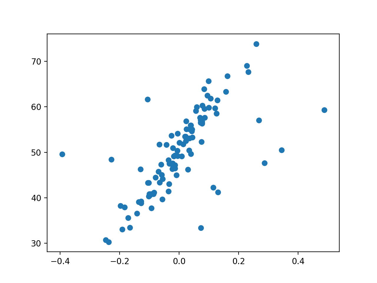
Running the example creates the synthetic regression dataset and adds outlier values.

The dataset is then plotted, and we can clearly see the linear relationship in the data, with statistical noise, and a modest number of outliers as points far from the main mass of data.

Scatter Plot of Regression Dataset With Outliers

Scatter Plot of Regression Dataset With Outliers

Now that we have a dataset, let’s fit different regression models on it.

Robust Regression Algorithms

In this section, we will consider different robust regression algorithms for the dataset.

Linear Regression (not robust)

Before diving into robust regression algorithms, let’s start with linear regression.

We can evaluate linear regression using repeated k-fold cross-validation on the regression dataset with outliers. We will measure mean absolute error and this will provide a lower bound on model performance on this task that we might expect some robust regression algorithms to out-perform.

# evaluate a model
def evaluate_model(X, y, model):
	# define model evaluation method
	cv = RepeatedKFold(n_splits=10, n_repeats=3, random_state=1)
	# evaluate model
	scores = cross_val_score(model, X, y, scoring='neg_mean_absolute_error', cv=cv, n_jobs=-1)
	# force scores to be positive
	return absolute(scores)

We can also plot the model’s line of best fit on the dataset. To do this, we first fit the model on the entire training dataset, then create an input dataset that is a grid across the entire input domain, make a prediction for each, then draw a line for the inputs and predicted outputs.

This plot shows how the model “sees” the problem, specifically the relationship between the input and output variables. The idea is that the line will be skewed by the outliers when using linear regression.

# plot the dataset and the model's line of best fit
def plot_best_fit(X, y, model):
	# fut the model on all data
	model.fit(X, y)
	# plot the dataset
	pyplot.scatter(X, y)
	# plot the line of best fit
	xaxis = arange(X.min(), X.max(), 0.01)
	yaxis = model.predict(xaxis.reshape((len(xaxis), 1)))
	pyplot.plot(xaxis, yaxis, color='r')
	# show the plot
	pyplot.title(type(model).__name__)
	pyplot.show()

Tying this together, the complete example for linear regression is listed below.

# linear regression on a dataset with outliers
from random import random
from random import randint
from random import seed
from numpy import arange
from numpy import mean
from numpy import std
from numpy import absolute
from sklearn.datasets import make_regression
from sklearn.linear_model import LinearRegression
from sklearn.model_selection import cross_val_score
from sklearn.model_selection import RepeatedKFold
from matplotlib import pyplot

# prepare the dataset
def get_dataset():
	X, y = make_regression(n_samples=100, n_features=1, tail_strength=0.9, effective_rank=1, n_informative=1, noise=3, bias=50, random_state=1)
	# add some artificial outliers
	seed(1)
	for i in range(10):
		factor = randint(2, 4)
		if random() > 0.5:
			X[i] += factor * X.std()
		else:
			X[i] -= factor * X.std()
	return X, y

# evaluate a model
def evaluate_model(X, y, model):
	# define model evaluation method
	cv = RepeatedKFold(n_splits=10, n_repeats=3, random_state=1)
	# evaluate model
	scores = cross_val_score(model, X, y, scoring='neg_mean_absolute_error', cv=cv, n_jobs=-1)
	# force scores to be positive
	return absolute(scores)

# plot the dataset and the model's line of best fit
def plot_best_fit(X, y, model):
	# fut the model on all data
	model.fit(X, y)
	# plot the dataset
	pyplot.scatter(X, y)
	# plot the line of best fit
	xaxis = arange(X.min(), X.max(), 0.01)
	yaxis = model.predict(xaxis.reshape((len(xaxis), 1)))
	pyplot.plot(xaxis, yaxis, color='r')
	# show the plot
	pyplot.title(type(model).__name__)
	pyplot.show()

# load dataset
X, y = get_dataset()
# define the model
model = LinearRegression()
# evaluate model
results = evaluate_model(X, y, model)
print('Mean MAE: %.3f (%.3f)' % (mean(results), std(results)))
# plot the line of best fit
plot_best_fit(X, y, model)

Running the example first reports the mean MAE for the model on the dataset.

We can see that linear regression achieves a MAE of about 5.2 on this dataset, providing an upper-bound in error.

Mean MAE: 5.260 (1.149)

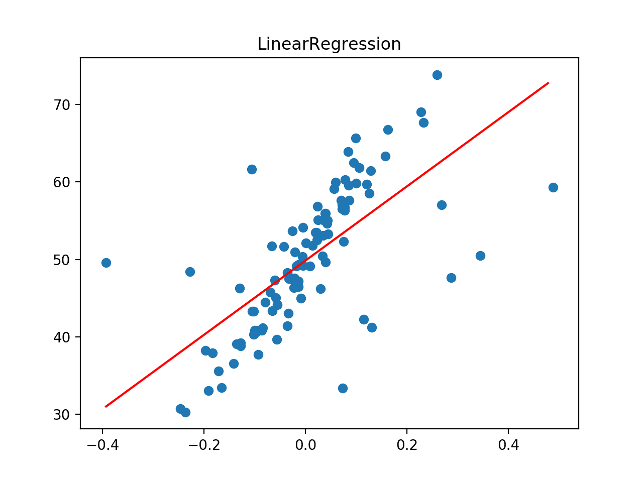
Next, the dataset is plotted as a scatter plot showing the outliers and this is overlaid with the line of best fit from the linear regression algorithm.

In this case, we can see that the line of best fit is not aligning with the data and it has been skewed by the outliers. In turn, we expect this has caused the model to have a worse-than-expected performance on the dataset.

Line of Best Fit for Linear Regression on a Dataset with Outliers

Line of Best Fit for Linear Regression on a Dataset with Outliers

Huber Regression

Huber regression is a type of robust regression that is aware of the possibility of outliers in a dataset and assigns them less weight than other examples in the dataset.

We can use Huber regression via the HuberRegressor class in scikit-learn. The “epsilon” argument controls what is considered an outlier, where smaller values consider more of the data outliers, and in turn, make the model more robust to outliers. The default is 1.35.

The example below evaluates Huber regression on the regression dataset with outliers, first evaluating the model with repeated cross-validation and then plotting the line of best fit.

# huber regression on a dataset with outliers
from random import random
from random import randint
from random import seed
from numpy import arange
from numpy import mean
from numpy import std
from numpy import absolute
from sklearn.datasets import make_regression
from sklearn.linear_model import HuberRegressor
from sklearn.model_selection import cross_val_score
from sklearn.model_selection import RepeatedKFold
from matplotlib import pyplot

# prepare the dataset
def get_dataset():
	X, y = make_regression(n_samples=100, n_features=1, tail_strength=0.9, effective_rank=1, n_informative=1, noise=3, bias=50, random_state=1)
	# add some artificial outliers
	seed(1)
	for i in range(10):
		factor = randint(2, 4)
		if random() > 0.5:
			X[i] += factor * X.std()
		else:
			X[i] -= factor * X.std()
	return X, y

# evaluate a model
def evaluate_model(X, y, model):
	# define model evaluation method
	cv = RepeatedKFold(n_splits=10, n_repeats=3, random_state=1)
	# evaluate model
	scores = cross_val_score(model, X, y, scoring='neg_mean_absolute_error', cv=cv, n_jobs=-1)
	# force scores to be positive
	return absolute(scores)

# plot the dataset and the model's line of best fit
def plot_best_fit(X, y, model):
	# fut the model on all data
	model.fit(X, y)
	# plot the dataset
	pyplot.scatter(X, y)
	# plot the line of best fit
	xaxis = arange(X.min(), X.max(), 0.01)
	yaxis = model.predict(xaxis.reshape((len(xaxis), 1)))
	pyplot.plot(xaxis, yaxis, color='r')
	# show the plot
	pyplot.title(type(model).__name__)
	pyplot.show()

# load dataset
X, y = get_dataset()
# define the model
model = HuberRegressor()
# evaluate model
results = evaluate_model(X, y, model)
print('Mean MAE: %.3f (%.3f)' % (mean(results), std(results)))
# plot the line of best fit
plot_best_fit(X, y, model)

Running the example first reports the mean MAE for the model on the dataset.

We can see that Huber regression achieves a MAE of about 4.435 on this dataset, outperforming the linear regression model in the previous section.

Mean MAE: 4.435 (1.868)

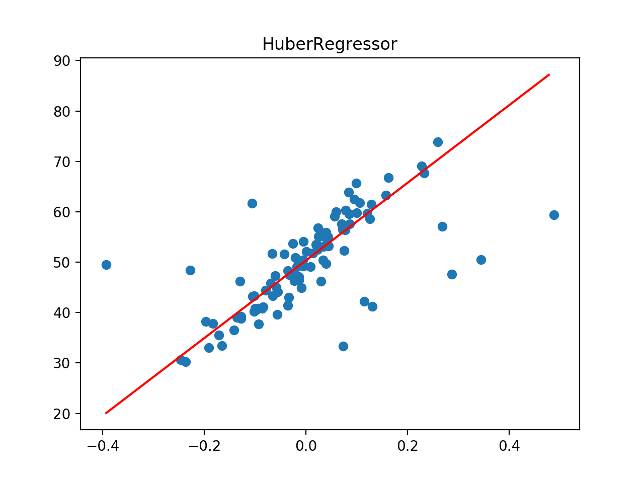
Next, the dataset is plotted as a scatter plot showing the outliers and this is overlaid with the line of best fit from the algorithm.

In this case, we can see that the line of best fit is better aligned with the main body of the data, and does not appear to be obviously influenced by the outliers that are present.

Line of Best Fit for Huber Regression on a Dataset with Outliers

Line of Best Fit for Huber Regression on a Dataset with Outliers

RANSAC Regression

Random Sample Consensus, or RANSAC for short, is another robust regression algorithm.

RANSAC tries to separate data into outliers and inliers and fits the model on the inliers.

The scikit-learn library provides an implementation via the RANSACRegressor class.

The example below evaluates RANSAC regression on the regression dataset with outliers, first evaluating the model with repeated cross-validation and then plotting the line of best fit.

# ransac regression on a dataset with outliers
from random import random
from random import randint
from random import seed
from numpy import arange
from numpy import mean
from numpy import std
from numpy import absolute
from sklearn.datasets import make_regression
from sklearn.linear_model import RANSACRegressor
from sklearn.model_selection import cross_val_score
from sklearn.model_selection import RepeatedKFold
from matplotlib import pyplot

# prepare the dataset
def get_dataset():
	X, y = make_regression(n_samples=100, n_features=1, tail_strength=0.9, effective_rank=1, n_informative=1, noise=3, bias=50, random_state=1)
	# add some artificial outliers
	seed(1)
	for i in range(10):
		factor = randint(2, 4)
		if random() > 0.5:
			X[i] += factor * X.std()
		else:
			X[i] -= factor * X.std()
	return X, y

# evaluate a model
def evaluate_model(X, y, model):
	# define model evaluation method
	cv = RepeatedKFold(n_splits=10, n_repeats=3, random_state=1)
	# evaluate model
	scores = cross_val_score(model, X, y, scoring='neg_mean_absolute_error', cv=cv, n_jobs=-1)
	# force scores to be positive
	return absolute(scores)

# plot the dataset and the model's line of best fit
def plot_best_fit(X, y, model):
	# fut the model on all data
	model.fit(X, y)
	# plot the dataset
	pyplot.scatter(X, y)
	# plot the line of best fit
	xaxis = arange(X.min(), X.max(), 0.01)
	yaxis = model.predict(xaxis.reshape((len(xaxis), 1)))
	pyplot.plot(xaxis, yaxis, color='r')
	# show the plot
	pyplot.title(type(model).__name__)
	pyplot.show()

# load dataset
X, y = get_dataset()
# define the model
model = RANSACRegressor()
# evaluate model
results = evaluate_model(X, y, model)
print('Mean MAE: %.3f (%.3f)' % (mean(results), std(results)))
# plot the line of best fit
plot_best_fit(X, y, model)

Running the example first reports the mean MAE for the model on the dataset.

We can see that RANSAC regression achieves a MAE of about 4.454 on this dataset, outperforming the linear regression model but perhaps not Huber regression.

Mean MAE: 4.454 (2.165)

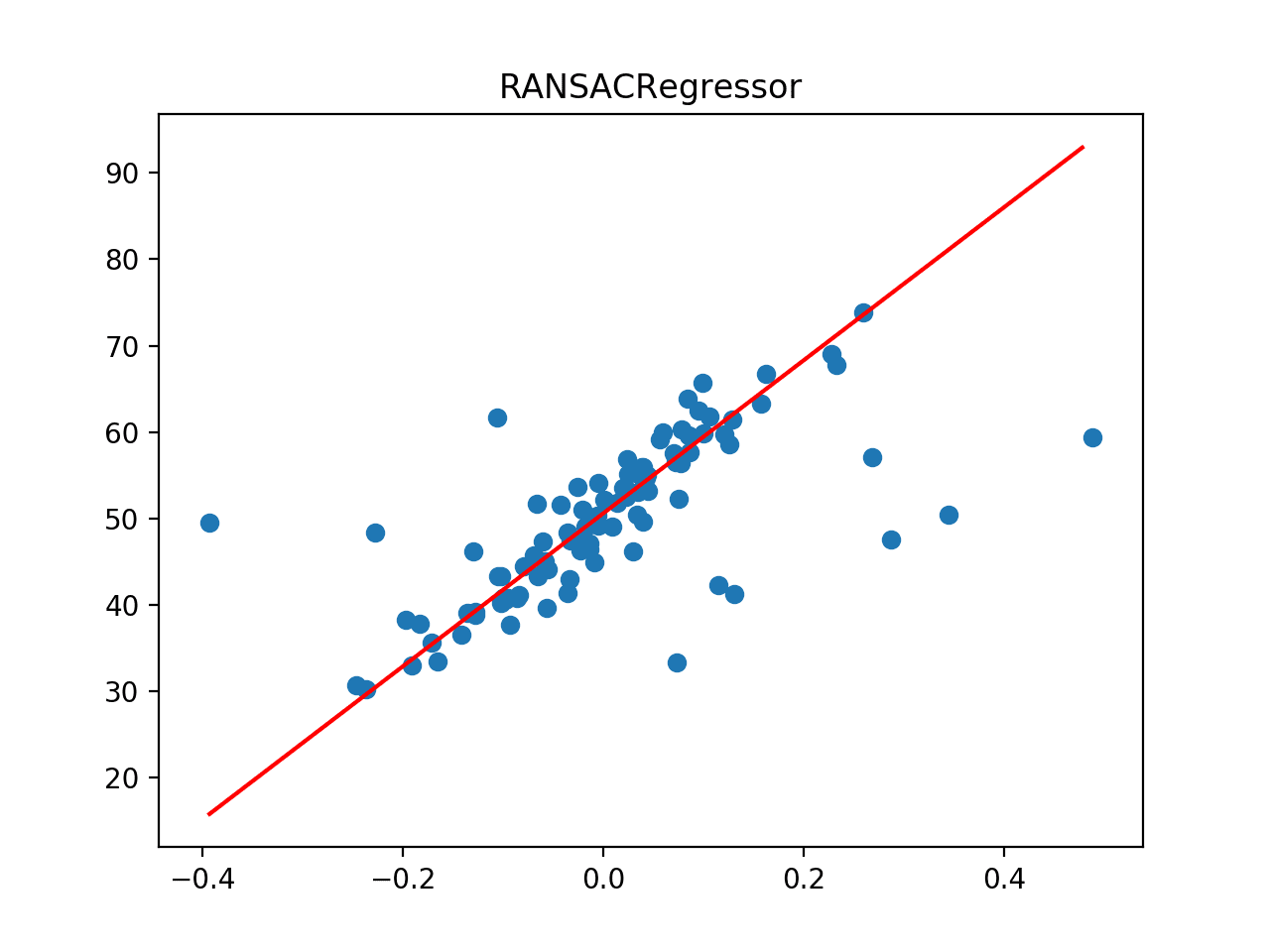
Next, the dataset is plotted as a scatter plot showing the outliers, and this is overlaid with the line of best fit from the algorithm.

In this case, we can see that the line of best fit is aligned with the main body of the data, perhaps even better than the plot for Huber regression.

Line of Best Fit for RANSAC Regression on a Dataset with Outliers

Line of Best Fit for RANSAC Regression on a Dataset with Outliers

Theil Sen Regression

Theil Sen regression involves fitting multiple regression models on subsets of the training data and combining the coefficients together in the end.

The scikit-learn provides an implementation via the TheilSenRegressor class.

The example below evaluates Theil Sen regression on the regression dataset with outliers, first evaluating the model with repeated cross-validation and then plotting the line of best fit.

# theilsen regression on a dataset with outliers
from random import random
from random import randint
from random import seed
from numpy import arange
from numpy import mean
from numpy import std
from numpy import absolute
from sklearn.datasets import make_regression
from sklearn.linear_model import TheilSenRegressor
from sklearn.model_selection import cross_val_score
from sklearn.model_selection import RepeatedKFold
from matplotlib import pyplot

# prepare the dataset
def get_dataset():
	X, y = make_regression(n_samples=100, n_features=1, tail_strength=0.9, effective_rank=1, n_informative=1, noise=3, bias=50, random_state=1)
	# add some artificial outliers
	seed(1)
	for i in range(10):
		factor = randint(2, 4)
		if random() > 0.5:
			X[i] += factor * X.std()
		else:
			X[i] -= factor * X.std()
	return X, y

# evaluate a model
def evaluate_model(X, y, model):
	# define model evaluation method
	cv = RepeatedKFold(n_splits=10, n_repeats=3, random_state=1)
	# evaluate model
	scores = cross_val_score(model, X, y, scoring='neg_mean_absolute_error', cv=cv, n_jobs=-1)
	# force scores to be positive
	return absolute(scores)

# plot the dataset and the model's line of best fit
def plot_best_fit(X, y, model):
	# fut the model on all data
	model.fit(X, y)
	# plot the dataset
	pyplot.scatter(X, y)
	# plot the line of best fit
	xaxis = arange(X.min(), X.max(), 0.01)
	yaxis = model.predict(xaxis.reshape((len(xaxis), 1)))
	pyplot.plot(xaxis, yaxis, color='r')
	# show the plot
	pyplot.title(type(model).__name__)
	pyplot.show()

# load dataset
X, y = get_dataset()
# define the model
model = TheilSenRegressor()
# evaluate model
results = evaluate_model(X, y, model)
print('Mean MAE: %.3f (%.3f)' % (mean(results), std(results)))
# plot the line of best fit
plot_best_fit(X, y, model)

Running the example first reports the mean MAE for the model on the dataset.

We can see that Theil Sen regression achieves a MAE of about 4.371 on this dataset, outperforming the linear regression model as well as RANSAC and Huber regression.

Mean MAE: 4.371 (1.961)

Next, the dataset is plotted as a scatter plot showing the outliers, and this is overlaid with the line of best fit from the algorithm.

In this case, we can see that the line of best fit is aligned with the main body of the data.

Line of Best Fit for Theil Sen Regression on a Dataset with Outliers

Line of Best Fit for Theil Sen Regression on a Dataset with Outliers

Compare Robust Regression Algorithms

Now that we are familiar with some popular robust regression algorithms and how to use them, we can look at how we might compare them directly.

It can be useful to run an experiment to directly compare the robust regression algorithms on the same dataset. We can compare the mean performance of each method, and more usefully, use tools like a box and whisker plot to compare the distribution of scores across the repeated cross-validation folds.

The complete example is listed below.

# compare robust regression algorithms on a regression dataset with outliers
from random import random
from random import randint
from random import seed
from numpy import mean
from numpy import std
from numpy import absolute
from sklearn.datasets import make_regression
from sklearn.model_selection import cross_val_score
from sklearn.model_selection import RepeatedKFold
from sklearn.linear_model import LinearRegression
from sklearn.linear_model import HuberRegressor
from sklearn.linear_model import RANSACRegressor
from sklearn.linear_model import TheilSenRegressor
from matplotlib import pyplot

# prepare the dataset
def get_dataset():
	X, y = make_regression(n_samples=100, n_features=1, tail_strength=0.9, effective_rank=1, n_informative=1, noise=3, bias=50, random_state=1)
	# add some artificial outliers
	seed(1)
	for i in range(10):
		factor = randint(2, 4)
		if random() > 0.5:
			X[i] += factor * X.std()
		else:
			X[i] -= factor * X.std()
	return X, y

# dictionary of model names and model objects
def get_models():
	models = dict()
	models['Linear'] = LinearRegression()
	models['Huber'] = HuberRegressor()
	models['RANSAC'] = RANSACRegressor()
	models['TheilSen'] = TheilSenRegressor()
	return models

# evaluate a model
def evalute_model(X, y, model, name):
	# define model evaluation method
	cv = RepeatedKFold(n_splits=10, n_repeats=3, random_state=1)
	# evaluate model
	scores = cross_val_score(model, X, y, scoring='neg_mean_absolute_error', cv=cv, n_jobs=-1)
	# force scores to be positive
	scores = absolute(scores)
	return scores

# load the dataset
X, y = get_dataset()
# retrieve models
models = get_models()
results = dict()
for name, model in models.items():
	# evaluate the model
	results[name] = evalute_model(X, y, model, name)
	# summarize progress
	print('>%s %.3f (%.3f)' % (name, mean(results[name]), std(results[name])))
# plot model performance for comparison
pyplot.boxplot(results.values(), labels=results.keys(), showmeans=True)
pyplot.show()

Running the example evaluates each model in turn, reporting the mean and standard deviation MAE scores of reach.

Note: your specific results will differ given the stochastic nature of the learning algorithms and evaluation procedure. Try running the example a few times.

We can see some minor differences between these scores and those reported in the previous section, although the differences may or may not be statistically significant. The general pattern of the robust regression methods performing better than linear regression holds, TheilSen achieving better performance than the other methods.

>Linear 5.260 (1.149)
>Huber 4.435 (1.868)
>RANSAC 4.405 (2.206)
>TheilSen 4.371 (1.961)

A plot is created showing a box and whisker plot summarizing the distribution of results for each evaluated algorithm.

We can clearly see the distributions for the robust regression algorithms sitting and extending lower than the linear regression algorithm.

Box and Whisker Plot of MAE Scores for Robust Regression Algorithms

Box and Whisker Plot of MAE Scores for Robust Regression Algorithms

It may also be interesting to compare robust regression algorithms based on a plot of their line of best fit.

The example below fits each robust regression algorithm and plots their line of best fit on the same plot in the context of a scatter plot of the entire training dataset.

# plot line of best for multiple robust regression algorithms
from random import random
from random import randint
from random import seed
from numpy import arange
from sklearn.datasets import make_regression
from sklearn.linear_model import LinearRegression
from sklearn.linear_model import HuberRegressor
from sklearn.linear_model import RANSACRegressor
from sklearn.linear_model import TheilSenRegressor
from matplotlib import pyplot

# prepare the dataset
def get_dataset():
	X, y = make_regression(n_samples=100, n_features=1, tail_strength=0.9, effective_rank=1, n_informative=1, noise=3, bias=50, random_state=1)
	# add some artificial outliers
	seed(1)
	for i in range(10):
		factor = randint(2, 4)
		if random() > 0.5:
			X[i] += factor * X.std()
		else:
			X[i] -= factor * X.std()
	return X, y

# dictionary of model names and model objects
def get_models():
	models = list()
	models.append(LinearRegression())
	models.append(HuberRegressor())
	models.append(RANSACRegressor())
	models.append(TheilSenRegressor())
	return models

# plot the dataset and the model's line of best fit
def plot_best_fit(X, y, xaxis, model):
	# fit the model on all data
	model.fit(X, y)
	# calculate outputs for grid across the domain
	yaxis = model.predict(xaxis.reshape((len(xaxis), 1)))
	# plot the line of best fit
	pyplot.plot(xaxis, yaxis, label=type(model).__name__)

# load the dataset
X, y = get_dataset()
# define a uniform grid across the input domain
xaxis = arange(X.min(), X.max(), 0.01)
for model in get_models():
	# plot the line of best fit
	plot_best_fit(X, y, xaxis, model)
# plot the dataset
pyplot.scatter(X, y)
# show the plot
pyplot.title('Robust Regression')
pyplot.legend()
pyplot.show()

Running the example creates a plot showing the dataset as a scatter plot and the line of best fit for each algorithm.

We can clearly see the off-axis line for the linear regression algorithm and the much better lines for the robust regression algorithms that follow the main body of the data.

Comparison of Robust Regression Algorithms Line of Best Fit

Comparison of Robust Regression Algorithms Line of Best Fit

Further Reading

This section provides more resources on the topic if you are looking to go deeper.

APIs

Articles

Summary

In this tutorial, you discovered robust regression algorithms for machine learning.

Specifically, you learned:

  • Robust regression algorithms can be used for data with outliers in the input or target values.
  • How to evaluate robust regression algorithms for a regression predictive modeling task.
  • How to compare robust regression algorithms using their line of best fit on the dataset.

Do you have any questions?
Ask your questions in the comments below and I will do my best to answer.

The post Robust Regression for Machine Learning in Python appeared first on Machine Learning Mastery.
How to Develop Elastic Net Regression Models in Python

$
0
0

Regression is a modeling task that involves predicting a numeric value given an input.

Linear regression is the standard algorithm for regression that assumes a linear relationship between inputs and the target variable. An extension to linear regression involves adding penalties to the loss function during training that encourage simpler models that have smaller coefficient values. These extensions are referred to as regularized linear regression or penalized linear regression.

Elastic net is a popular type of regularized linear regression that combines two popular penalties, specifically the L1 and L2 penalty functions.

In this tutorial, you will discover how to develop Elastic Net regularized regression in Python.

After completing this tutorial, you will know:

  • Elastic Net is an extension of linear regression that adds regularization penalties to the loss function during training.
  • How to evaluate an Elastic Net model and use a final model to make predictions for new data.
  • How to configure the Elastic Net model for a new dataset via grid search and automatically.

Let’s get started.

How to Develop Elastic Net Regression Models in Python

How to Develop Elastic Net Regression Models in Python
Photo by Phil Dolby, some rights reserved.

Tutorial Overview

This tutorial is divided into three parts; they are:

  1. Elastic Net Regression
  2. Example of Elastic Net Regression
  3. Tuning Elastic Net Hyperparameters

Elastic Net Regression

Linear regression refers to a model that assumes a linear relationship between input variables and the target variable.

With a single input variable, this relationship is a line, and with higher dimensions, this relationship can be thought of as a hyperplane that connects the input variables to the target variable. The coefficients of the model are found via an optimization process that seeks to minimize the sum squared error between the predictions (yhat) and the expected target values (y).

  • loss = sum i=0 to n (y_i – yhat_i)^2

A problem with linear regression is that estimated coefficients of the model can become large, making the model sensitive to inputs and possibly unstable. This is particularly true for problems with few observations (samples) or more samples (n) than input predictors (p) or variables (so-called p >> n problems).

One approach to addressing the stability of regression models is to change the loss function to include additional costs for a model that has large coefficients. Linear regression models that use these modified loss functions during training are referred to collectively as penalized linear regression.

One popular penalty is to penalize a model based on the sum of the squared coefficient values. This is called an L2 penalty. An L2 penalty minimizes the size of all coefficients, although it prevents any coefficients from being removed from the model.

  • l2_penalty = sum j=0 to p beta_j^2

Another popular penalty is to penalize a model based on the sum of the absolute coefficient values. This is called the L1 penalty. An L1 penalty minimizes the size of all coefficients and allows some coefficients to be minimized to the value zero, which removes the predictor from the model.

  • l1_penalty = sum j=0 to p abs(beta_j)

Elastic net is a penalized linear regression model that includes both the L1 and L2 penalties during training.

Using the terminology from “The Elements of Statistical Learning,” a hyperparameter “alpha” is provided to assign how much weight is given to each of the L1 and L2 penalties. Alpha is a value between 0 and 1 and is used to weight the contribution of the L1 penalty and one minus the alpha value is used to weight the L2 penalty.

  • elastic_net_penalty = (alpha * l1_penalty) + ((1 – alpha) * l2_penalty)

For example, an alpha of 0.5 would provide a 50 percent contribution of each penalty to the loss function. An alpha value of 0 gives all weight to the L2 penalty and a value of 1 gives all weight to the L1 penalty.

The parameter alpha determines the mix of the penalties, and is often pre-chosen on qualitative grounds.

— Page 663, The Elements of Statistical Learning, 2016.

The benefit is that elastic net allows a balance of both penalties, which can result in better performance than a model with either one or the other penalty on some problems.

Another hyperparameter is provided called “lambda” that controls the weighting of the sum of both penalties to the loss function. A default value of 1.0 is used to use the fully weighted penalty; a value of 0 excludes the penalty. Very small values of lambada, such as 1e-3 or smaller, are common.

  • elastic_net_loss = loss + (lambda * elastic_net_penalty)

Now that we are familiar with elastic net penalized regression, let’s look at a worked example.

Example of Elastic Net Regression

In this section, we will demonstrate how to use the Elastic Net regression algorithm.

First, let’s introduce a standard regression dataset. We will use the housing dataset.

The housing dataset is a standard machine learning dataset comprising 506 rows of data with 13 numerical input variables and a numerical target variable.

Using a test harness of repeated stratified 10-fold cross-validation with three repeats, a naive model can achieve a mean absolute error (MAE) of about 6.6. A top-performing model can achieve a MAE on this same test harness of about 1.9. This provides the bounds of expected performance on this dataset.

The dataset involves predicting the house price given details of the house’s suburb in the American city of Boston.

No need to download the dataset; we will download it automatically as part of our worked examples.

The example below downloads and loads the dataset as a Pandas DataFrame and summarizes the shape of the dataset and the first five rows of data.

# load and summarize the housing dataset
from pandas import read_csv
from matplotlib import pyplot
# load dataset
url = 'https://raw.githubusercontent.com/jbrownlee/Datasets/master/housing.csv'
dataframe = read_csv(url, header=None)
# summarize shape
print(dataframe.shape)
# summarize first few lines
print(dataframe.head())

Running the example confirms the 506 rows of data and 13 input variables and a single numeric target variable (14 in total).

We can also see that all input variables are numeric.

(506, 14)
        0     1     2   3      4      5   ...  8      9     10      11    12    13
0  0.00632  18.0  2.31   0  0.538  6.575  ...   1  296.0  15.3  396.90  4.98  24.0
1  0.02731   0.0  7.07   0  0.469  6.421  ...   2  242.0  17.8  396.90  9.14  21.6
2  0.02729   0.0  7.07   0  0.469  7.185  ...   2  242.0  17.8  392.83  4.03  34.7
3  0.03237   0.0  2.18   0  0.458  6.998  ...   3  222.0  18.7  394.63  2.94  33.4
4  0.06905   0.0  2.18   0  0.458  7.147  ...   3  222.0  18.7  396.90  5.33  36.2

[5 rows x 14 columns]

The scikit-learn Python machine learning library provides an implementation of the Elastic Net penalized regression algorithm via the ElasticNet class.

Confusingly, the alpha hyperparameter can be set via the “l1_ratio” argument that controls the contribution of the L1 and L2 penalties and the lambda hyperparameter can be set via the “alpha” argument that controls the contribution of the sum of both penalties to the loss function.

By default, an equal balance of 0.5 is used for “l1_ratio” and a full weighting of 1.0 is used for alpha.

...
# define model
model = ElasticNet(alpha=1.0, l1_ratio=0.5)

We can evaluate the Elastic Net model on the housing dataset using repeated 10-fold cross-validation and report the average mean absolute error (MAE) on the dataset.

# evaluate an elastic net model on the dataset
from numpy import mean
from numpy import std
from numpy import absolute
from pandas import read_csv
from sklearn.model_selection import cross_val_score
from sklearn.model_selection import RepeatedKFold
from sklearn.linear_model import ElasticNet
# load the dataset
url = 'https://raw.githubusercontent.com/jbrownlee/Datasets/master/housing.csv'
dataframe = read_csv(url, header=None)
data = dataframe.values
X, y = data[:, :-1], data[:, -1]
# define model
model = ElasticNet(alpha=1.0, l1_ratio=0.5)
# define model evaluation method
cv = RepeatedKFold(n_splits=10, n_repeats=3, random_state=1)
# evaluate model
scores = cross_val_score(model, X, y, scoring='neg_mean_absolute_error', cv=cv, n_jobs=-1)
# force scores to be positive
scores = absolute(scores)
print('Mean MAE: %.3f (%.3f)' % (mean(scores), std(scores)))

Running the example evaluates the Elastic Net algorithm on the housing dataset and reports the average MAE across the three repeats of 10-fold cross-validation.

Your specific results may vary given the stochastic nature of the learning algorithm. Consider running the example a few times.

In this case, we can see that the model achieved a MAE of about 3.682.

Mean MAE: 3.682 (0.530)

We may decide to use the Elastic Net as our final model and make predictions on new data.

This can be achieved by fitting the model on all available data and calling the predict() function, passing in a new row of data.

We can demonstrate this with a complete example, listed below.

# make a prediction with an elastic net model on the dataset
from pandas import read_csv
from sklearn.linear_model import ElasticNet
# load the dataset
url = 'https://raw.githubusercontent.com/jbrownlee/Datasets/master/housing.csv'
dataframe = read_csv(url, header=None)
data = dataframe.values
X, y = data[:, :-1], data[:, -1]
# define model
model = ElasticNet(alpha=1.0, l1_ratio=0.5)
# fit model
model.fit(X, y)
# define new data
row = [0.00632,18.00,2.310,0,0.5380,6.5750,65.20,4.0900,1,296.0,15.30,396.90,4.98]
# make a prediction
yhat = model.predict([row])
# summarize prediction
print('Predicted: %.3f' % yhat)

Running the example fits the model and makes a prediction for the new rows of data.

Predicted: 31.047

Next, we can look at configuring the model hyperparameters.

Tuning Elastic Net Hyperparameters

How do we know that the default hyperparameters of alpha=1.0 and l1_ratio=0.5 are any good for our dataset?

We don’t.

Instead, it is good practice to test a suite of different configurations and discover what works best.

One approach would be to gird search l1_ratio values between 0 and 1 with a 0.1 or 0.01 separation and alpha values from perhaps 1e-5 to 100 on a log-10 scale and discover what works best for a dataset.

The example below demonstrates this using the GridSearchCV class with a grid of values we have defined.

# grid search hyperparameters for the elastic net
from numpy import arange
from pandas import read_csv
from sklearn.model_selection import GridSearchCV
from sklearn.model_selection import RepeatedKFold
from sklearn.linear_model import ElasticNet
# load the dataset
url = 'https://raw.githubusercontent.com/jbrownlee/Datasets/master/housing.csv'
dataframe = read_csv(url, header=None)
data = dataframe.values
X, y = data[:, :-1], data[:, -1]
# define model
model = ElasticNet()
# define model evaluation method
cv = RepeatedKFold(n_splits=10, n_repeats=3, random_state=1)
# define grid
grid = dict()
grid['alpha'] = [1e-5, 1e-4, 1e-3, 1e-2, 1e-1, 0.0, 1.0, 10.0, 100.0]
grid['l1_ratio'] = arange(0, 1, 0.01)
# define search
search = GridSearchCV(model, grid, scoring='neg_mean_absolute_error', cv=cv, n_jobs=-1)
# perform the search
results = search.fit(X, y)
# summarize
print('MAE: %.3f' % results.best_score_)
print('Config: %s' % results.best_params_)

Running the example will evaluate each combination of configurations using repeated cross-validation.

You might see some warnings that can be safely ignored, such as:

Objective did not converge. You might want to increase the number of iterations.

Your specific results may vary given the stochastic nature of the learning algorithm. Try running the example a few times.

In this case, we can see that we achieved slightly better results than the default 3.378 vs. 3.682. Ignore the sign; the library makes the MAE negative for optimization purposes.

We can see that the model assigned an alpha weight of 0.01 to the penalty and focuses exclusively on the L2 penalty.

MAE: -3.378
Config: {'alpha': 0.01, 'l1_ratio': 0.97}

The scikit-learn library also provides a built-in version of the algorithm that automatically finds good hyperparameters via the ElasticNetCV class.

To use this class, it is first fit on the dataset, then used to make a prediction. It will automatically find appropriate hyperparameters.

By default, the model will test 100 alpha values and use a default ratio. We can specify our own lists of values to test via the “l1_ratio” and “alphas” arguments, as we did with the manual grid search.

The example below demonstrates this.

# use automatically configured elastic net algorithm
from numpy import arange
from pandas import read_csv
from sklearn.linear_model import ElasticNetCV
from sklearn.model_selection import RepeatedKFold
# load the dataset
url = 'https://raw.githubusercontent.com/jbrownlee/Datasets/master/housing.csv'
dataframe = read_csv(url, header=None)
data = dataframe.values
X, y = data[:, :-1], data[:, -1]
# define model evaluation method
cv = RepeatedKFold(n_splits=10, n_repeats=3, random_state=1)
# define model
ratios = arange(0, 1, 0.01)
alphas = [1e-5, 1e-4, 1e-3, 1e-2, 1e-1, 0.0, 1.0, 10.0, 100.0]
model = ElasticNetCV(l1_ratio=ratios, alphas=alphas, cv=cv, n_jobs=-1)
# fit model
model.fit(X, y)
# summarize chosen configuration
print('alpha: %f' % model.alpha_)
print('l1_ratio_: %f' % model.l1_ratio_)

Your specific results may vary given the stochastic nature of the learning algorithm. Try running the example a few times.

Again, you might see some warnings that can be safely ignored, such as:

Objective did not converge. You might want to increase the number of iterations.

In this case, we can see that an alpha of 0.0 was chosen, removing both penalties from the loss function.

This is different from what we found via our manual grid search, perhaps due to the systematic way in which configurations were searched or selected.

alpha: 0.000000
l1_ratio_: 0.470000

Further Reading

This section provides more resources on the topic if you are looking to go deeper.

Books

APIs

Articles

Summary

In this tutorial, you discovered how to develop Elastic Net regularized regression in Python.

Specifically, you learned:

  • Elastic Net is an extension of linear regression that adds regularization penalties to the loss function during training.
  • How to evaluate an Elastic Net model and use a final model to make predictions for new data.
  • How to configure the Elastic Net model for a new dataset via grid search and automatically.

Do you have any questions?
Ask your questions in the comments below and I will do my best to answer.

The post How to Develop Elastic Net Regression Models in Python appeared first on Machine Learning Mastery.
How to Develop Ridge Regression Models in Python

$
0
0

Regression is a modeling task that involves predicting a numeric value given an input.

Linear regression is the standard algorithm for regression that assumes a linear relationship between inputs and the target variable. An extension to linear regression invokes adding penalties to the loss function during training that encourages simpler models that have smaller coefficient values. These extensions are referred to as regularized linear regression or penalized linear regression.

Ridge Regression is a popular type of regularized linear regression that includes an L2 penalty. This has the effect of shrinking the coefficients for those input variables that do not contribute much to the prediction task.

In this tutorial, you will discover how to develop and evaluate Ridge Regression models in Python.

After completing this tutorial, you will know:

  • Ridge Regression is an extension of linear regression that adds a regularization penalty to the loss function during training.
  • How to evaluate a Ridge Regression model and use a final model to make predictions for new data.
  • How to configure the Ridge Regression model for a new dataset via grid search and automatically.

Let’s get started.

How to Develop Ridge Regression Models in Python

How to Develop Ridge Regression Models in Python
Photo by Susanne Nilsson, some rights reserved.

Tutorial Overview

This tutorial is divided into three parts; they are:

  1. Ridge Regression
  2. Example of Ridge Regression
  3. Tuning Ridge Hyperparameters

Ridge Regression

Linear regression refers to a model that assumes a linear relationship between input variables and the target variable.

With a single input variable, this relationship is a line, and with higher dimensions, this relationship can be thought of as a hyperplane that connects the input variables to the target variable. The coefficients of the model are found via an optimization process that seeks to minimize the sum squared error between the predictions (yhat) and the expected target values (y).

  • loss = sum i=0 to n (y_i – yhat_i)^2

A problem with linear regression is that estimated coefficients of the model can become large, making the model sensitive to inputs and possibly unstable. This is particularly true for problems with few observations (samples) or more samples (n) than input predictors (p) or variables (so-called p >> n problems).

One approach to address the stability of regression models is to change the loss function to include additional costs for a model that has large coefficients. Linear regression models that use these modified loss functions during training are referred to collectively as penalized linear regression.

One popular penalty is to penalize a model based on the sum of the squared coefficient values (beta). This is called an L2 penalty.

  • l2_penalty = sum j=0 to p beta_j^2

An L2 penalty minimizes the size of all coefficients, although it prevents any coefficients from being removed from the model by allowing their value to become zero.

The effect of this penalty is that the parameter estimates are only allowed to become large if there is a proportional reduction in SSE. In effect, this method shrinks the estimates towards 0 as the lambda penalty becomes large (these techniques are sometimes called “shrinkage methods”).

— Page 123, Applied Predictive Modeling, 2013.

This penalty can be added to the cost function for linear regression and is referred to as Tikhonov regularization (after the author), or Ridge Regression more generally.

A hyperparameter is used called “lambda” that controls the weighting of the penalty to the loss function. A default value of 1.0 will fully weight the penalty; a value of 0 excludes the penalty. Very small values of lambda, such as 1e-3 or smaller are common.

  • ridge_loss = loss + (lambda * l2_penalty)

Now that we are familiar with Ridge penalized regression, let’s look at a worked example.

Example of Ridge Regression

In this section, we will demonstrate how to use the Ridge Regression algorithm.

First, let’s introduce a standard regression dataset. We will use the housing dataset.

The housing dataset is a standard machine learning dataset comprising 506 rows of data with 13 numerical input variables and a numerical target variable.

Using a test harness of repeated stratified 10-fold cross-validation with three repeats, a naive model can achieve a mean absolute error (MAE) of about 6.6. A top-performing model can achieve a MAE on this same test harness of about 1.9. This provides the bounds of expected performance on this dataset.

The dataset involves predicting the house price given details of the house’s suburb in the American city of Boston.

No need to download the dataset; we will download it automatically as part of our worked examples.

The example below downloads and loads the dataset as a Pandas DataFrame and summarizes the shape of the dataset and the first five rows of data.

# load and summarize the housing dataset
from pandas import read_csv
from matplotlib import pyplot
# load dataset
url = 'https://raw.githubusercontent.com/jbrownlee/Datasets/master/housing.csv'
dataframe = read_csv(url, header=None)
# summarize shape
print(dataframe.shape)
# summarize first few lines
print(dataframe.head())

Running the example confirms the 506 rows of data and 13 input variables and a single numeric target variable (14 in total). We can also see that all input variables are numeric.

(506, 14)
        0     1     2   3      4      5   ...  8      9     10      11    12    13
0  0.00632  18.0  2.31   0  0.538  6.575  ...   1  296.0  15.3  396.90  4.98  24.0
1  0.02731   0.0  7.07   0  0.469  6.421  ...   2  242.0  17.8  396.90  9.14  21.6
2  0.02729   0.0  7.07   0  0.469  7.185  ...   2  242.0  17.8  392.83  4.03  34.7
3  0.03237   0.0  2.18   0  0.458  6.998  ...   3  222.0  18.7  394.63  2.94  33.4
4  0.06905   0.0  2.18   0  0.458  7.147  ...   3  222.0  18.7  396.90  5.33  36.2

[5 rows x 14 columns]

The scikit-learn Python machine learning library provides an implementation of the Ridge Regression algorithm via the Ridge class.

Confusingly, the lambda term can be configured via the “alpha” argument when defining the class. The default value is 1.0 or a full penalty.

...
# define model
model = Ridge(alpha=1.0)

We can evaluate the Ridge Regression model on the housing dataset using repeated 10-fold cross-validation and report the average mean absolute error (MAE) on the dataset.

# evaluate an ridge regression model on the dataset
from numpy import mean
from numpy import std
from numpy import absolute
from pandas import read_csv
from sklearn.model_selection import cross_val_score
from sklearn.model_selection import RepeatedKFold
from sklearn.linear_model import Ridge
# load the dataset
url = 'https://raw.githubusercontent.com/jbrownlee/Datasets/master/housing.csv'
dataframe = read_csv(url, header=None)
data = dataframe.values
X, y = data[:, :-1], data[:, -1]
# define model
model = Ridge(alpha=1.0)
# define model evaluation method
cv = RepeatedKFold(n_splits=10, n_repeats=3, random_state=1)
# evaluate model
scores = cross_val_score(model, X, y, scoring='neg_mean_absolute_error', cv=cv, n_jobs=-1)
# force scores to be positive
scores = absolute(scores)
print('Mean MAE: %.3f (%.3f)' % (mean(scores), std(scores)))

Running the example evaluates the Ridge Regression algorithm on the housing dataset and reports the average MAE across the three repeats of 10-fold cross-validation.

Your specific results may vary given the stochastic nature of the learning algorithm. Consider running the example a few times.

In this case, we can see that the model achieved a MAE of about 3.382.

Mean MAE: 3.382 (0.519)

We may decide to use the Ridge Regression as our final model and make predictions on new data.

This can be achieved by fitting the model on all available data and calling the predict() function, passing in a new row of data.

We can demonstrate this with a complete example listed below.

# make a prediction with a ridge regression model on the dataset
from pandas import read_csv
from sklearn.linear_model import Ridge
# load the dataset
url = 'https://raw.githubusercontent.com/jbrownlee/Datasets/master/housing.csv'
dataframe = read_csv(url, header=None)
data = dataframe.values
X, y = data[:, :-1], data[:, -1]
# define model
model = Ridge(alpha=1.0)
# fit model
model.fit(X, y)
# define new data
row = [0.00632,18.00,2.310,0,0.5380,6.5750,65.20,4.0900,1,296.0,15.30,396.90,4.98]
# make a prediction
yhat = model.predict([row])
# summarize prediction
print('Predicted: %.3f' % yhat)

Running the example fits the model and makes a prediction for the new rows of data.

Predicted: 30.253

Next, we can look at configuring the model hyperparameters.

Tuning Ridge Hyperparameters

How do we know that the default hyperparameters of alpha=1.0 is appropriate for our dataset?

We don’t.

Instead, it is good practice to test a suite of different configurations and discover what works best for our dataset.

One approach would be to grid search alpha values from perhaps 1e-5 to 100 on a log scale and discover what works best for a dataset. Another approach would be to test values between 0.0 and 1.0 with a grid separation of 0.01. We will try the latter in this case.

The example below demonstrates this using the GridSearchCV class with a grid of values we have defined.

# grid search hyperparameters for ridge regression
from numpy import arange
from pandas import read_csv
from sklearn.model_selection import GridSearchCV
from sklearn.model_selection import RepeatedKFold
from sklearn.linear_model import Ridge
# load the dataset
url = 'https://raw.githubusercontent.com/jbrownlee/Datasets/master/housing.csv'
dataframe = read_csv(url, header=None)
data = dataframe.values
X, y = data[:, :-1], data[:, -1]
# define model
model = Ridge()
# define model evaluation method
cv = RepeatedKFold(n_splits=10, n_repeats=3, random_state=1)
# define grid
grid = dict()
grid['alpha'] = [1e-5, 1e-4, 1e-3, 1e-2, 1e-1, 0.0, 1.0, 10.0, 100.0]
# define search
search = GridSearchCV(model, grid, scoring='neg_mean_absolute_error', cv=cv, n_jobs=-1)
# perform the search
results = search.fit(X, y)
# summarize
print('MAE: %.3f' % results.best_score_)
print('Config: %s' % results.best_params_)

Running the example will evaluate each combination of configurations using repeated cross-validation.

Your specific results may vary given the stochastic nature of the learning algorithm. Try running the example a few times.

In this case, we can see that we achieved slightly better results than the default 3.379 vs. 3.382. Ignore the sign; the library makes the MAE negative for optimization purposes.

We can see that the model assigned an alpha weight of 0.51 to the penalty.

MAE: -3.379
Config: {'alpha': 0.51}

The scikit-learn library also provides a built-in version of the algorithm that automatically finds good hyperparameters via the RidgeCV class.

To use this class, it is fit on the training dataset and used to make a prediction. During the training process, it automatically tunes the hyperparameter values.

By default, the model will only test the alpha values (0.1, 1.0, 10.0). We can change this to a grid of values between 0 and 1 with a separation of 0.01 as we did on the previous example by setting the “alphas” argument.

The example below demonstrates this.

# use automatically configured the ridge regression algorithm
from numpy import arange
from pandas import read_csv
from sklearn.linear_model import RidgeCV
from sklearn.model_selection import RepeatedKFold
# load the dataset
url = 'https://raw.githubusercontent.com/jbrownlee/Datasets/master/housing.csv'
dataframe = read_csv(url, header=None)
data = dataframe.values
X, y = data[:, :-1], data[:, -1]
# define model evaluation method
cv = RepeatedKFold(n_splits=10, n_repeats=3, random_state=1)
# define model
model = RidgeCV(alphas=arange(0, 1, 0.01), cv=cv, scoring='neg_mean_absolute_error')
# fit model
model.fit(X, y)
# summarize chosen configuration
print('alpha: %f' % model.alpha_)

Running the example fits the model and discovers the hyperparameters that give the best results using cross-validation.

Your specific results may vary given the stochastic nature of the learning algorithm. Try running the example a few times.

In this case, we can see that the model chose the identical hyperparameter of alpha=0.51 that we found via our manual grid search.

alpha: 0.510000

Further Reading

This section provides more resources on the topic if you are looking to go deeper.

Books

APIs

Articles

Summary

In this tutorial, you discovered how to develop and evaluate Ridge Regression models in Python.

Specifically, you learned:

  • Ridge Regression is an extension of linear regression that adds a regularization penalty to the loss function during training.
  • How to evaluate a Ridge Regression model and use a final model to make predictions for new data.
  • How to configure the Ridge Regression model for a new dataset via grid search and automatically.

Do you have any questions?
Ask your questions in the comments below and I will do my best to answer.

The post How to Develop Ridge Regression Models in Python appeared first on Machine Learning Mastery.
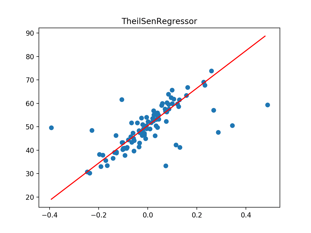
How to Develop LASSO Regression Models in Python

$
0
0

Regression is a modeling task that involves predicting a numeric value given an input.

Linear regression is the standard algorithm for regression that assumes a linear relationship between inputs and the target variable. An extension to linear regression invokes adding penalties to the loss function during training that encourages simpler models that have smaller coefficient values. These extensions are referred to as regularized linear regression or penalized linear regression.

Lasso Regression is a popular type of regularized linear regression that includes an L1 penalty. This has the effect of shrinking the coefficients for those input variables that do not contribute much to the prediction task. This penalty allows some coefficient values to go to the value of zero, allowing input variables to be effectively removed from the model, providing a type of automatic feature selection.

In this tutorial, you will discover how to develop and evaluate Lasso Regression models in Python.

After completing this tutorial, you will know:

  • Lasso Regression is an extension of linear regression that adds a regularization penalty to the loss function during training.
  • How to evaluate a Lasso Regression model and use a final model to make predictions for new data.
  • How to configure the Lasso Regression model for a new dataset via grid search and automatically.

Let’s get started.

How to Develop LASSO Regression Models in Python

How to Develop LASSO Regression Models in Python
Photo by Phil Dolby, some rights reserved.

Tutorial Overview

This tutorial is divided into three parts; they are:

  1. Lasso Regression
  2. Example of Lasso Regression
  3. Tuning Lasso Hyperparameters

Lasso Regression

Linear regression refers to a model that assumes a linear relationship between input variables and the target variable.

With a single input variable, this relationship is a line, and with higher dimensions, this relationship can be thought of as a hyperplane that connects the input variables to the target variable. The coefficients of the model are found via an optimization process that seeks to minimize the sum squared error between the predictions (yhat) and the expected target values (y).

  • loss = sum i=0 to n (y_i – yhat_i)^2

A problem with linear regression is that estimated coefficients of the model can become large, making the model sensitive to inputs and possibly unstable. This is particularly true for problems with few observations (samples) or more samples (n) than input predictors (p) or variables (so-called p >> n problems).

One approach to address the stability of regression models is to change the loss function to include additional costs for a model that has large coefficients. Linear regression models that use these modified loss functions during training are referred to collectively as penalized linear regression.

A popular penalty is to penalize a model based on the sum of the absolute coefficient values. This is called the L1 penalty. An L1 penalty minimizes the size of all coefficients and allows some coefficients to be minimized to the value zero, which removes the predictor from the model.

  • l1_penalty = sum j=0 to p abs(beta_j)

An L1 penalty minimizes the size of all coefficients and allows any coefficient to go to the value of zero, effectively removing input features from the model.

This acts as a type of automatic feature selection.

… a consequence of penalizing the absolute values is that some parameters are actually set to 0 for some value of lambda. Thus the lasso yields models that simultaneously use regularization to improve the model and to conduct feature selection.

— Page 125, Applied Predictive Modeling, 2013.

This penalty can be added to the cost function for linear regression and is referred to as Least Absolute Shrinkage And Selection Operator regularization (LASSO), or more commonly, “Lasso” (with title case) for short.

A popular alternative to ridge regression is the least absolute shrinkage and selection operator model, frequently called the lasso.

— Page 124, Applied Predictive Modeling, 2013.

A hyperparameter is used called “lambda” that controls the weighting of the penalty to the loss function. A default value of 1.0 will give full weightings to the penalty; a value of 0 excludes the penalty. Very small values of lambda, such as 1e-3 or smaller, are common.

  • lasso_loss = loss + (lambda * l1_penalty)

Now that we are familiar with Lasso penalized regression, let’s look at a worked example.

Example of Lasso Regression

In this section, we will demonstrate how to use the Lasso Regression algorithm.

First, let’s introduce a standard regression dataset. We will use the housing dataset.

The housing dataset is a standard machine learning dataset comprising 506 rows of data with 13 numerical input variables and a numerical target variable.

Using a test harness of repeated stratified 10-fold cross-validation with three repeats, a naive model can achieve a mean absolute error (MAE) of about 6.6. A top-performing model can achieve a MAE on this same test harness of about 1.9. This provides the bounds of expected performance on this dataset.

The dataset involves predicting the house price given details of the house suburb in the American city of Boston.

No need to download the dataset; we will download it automatically as part of our worked examples.

The example below downloads and loads the dataset as a Pandas DataFrame and summarizes the shape of the dataset and the first five rows of data.

# load and summarize the housing dataset
from pandas import read_csv
from matplotlib import pyplot
# load dataset
url = 'https://raw.githubusercontent.com/jbrownlee/Datasets/master/housing.csv'
dataframe = read_csv(url, header=None)
# summarize shape
print(dataframe.shape)
# summarize first few lines
print(dataframe.head())

Running the example confirms the 506 rows of data and 13 input variables and a single numeric target variable (14 in total). We can also see that all input variables are numeric.

(506, 14)
        0     1     2   3      4      5   ...  8      9     10      11    12    13
0  0.00632  18.0  2.31   0  0.538  6.575  ...   1  296.0  15.3  396.90  4.98  24.0
1  0.02731   0.0  7.07   0  0.469  6.421  ...   2  242.0  17.8  396.90  9.14  21.6
2  0.02729   0.0  7.07   0  0.469  7.185  ...   2  242.0  17.8  392.83  4.03  34.7
3  0.03237   0.0  2.18   0  0.458  6.998  ...   3  222.0  18.7  394.63  2.94  33.4
4  0.06905   0.0  2.18   0  0.458  7.147  ...   3  222.0  18.7  396.90  5.33  36.2

[5 rows x 14 columns]

The scikit-learn Python machine learning library provides an implementation of the Lasso penalized regression algorithm via the Lasso class.

Confusingly, the lambda term can be configured via the “alpha” argument when defining the class. The default value is 1.0 or a full penalty.

...
# define model
model = Lasso(alpha=1.0)

We can evaluate the Lasso Regression model on the housing dataset using repeated 10-fold cross-validation and report the average mean absolute error (MAE) on the dataset.

# evaluate an lasso regression model on the dataset
from numpy import mean
from numpy import std
from numpy import absolute
from pandas import read_csv
from sklearn.model_selection import cross_val_score
from sklearn.model_selection import RepeatedKFold
from sklearn.linear_model import Lasso
# load the dataset
url = 'https://raw.githubusercontent.com/jbrownlee/Datasets/master/housing.csv'
dataframe = read_csv(url, header=None)
data = dataframe.values
X, y = data[:, :-1], data[:, -1]
# define model
model = Lasso(alpha=1.0)
# define model evaluation method
cv = RepeatedKFold(n_splits=10, n_repeats=3, random_state=1)
# evaluate model
scores = cross_val_score(model, X, y, scoring='neg_mean_absolute_error', cv=cv, n_jobs=-1)
# force scores to be positive
scores = absolute(scores)
print('Mean MAE: %.3f (%.3f)' % (mean(scores), std(scores)))

Running the example evaluates the Lasso Regression algorithm on the housing dataset and reports the average MAE across the three repeats of 10-fold cross-validation.

Your specific results may vary given the stochastic nature of the learning algorithm. Consider running the example a few times.

In this case, we can see that the model achieved a MAE of about 3.711.

Mean MAE: 3.711 (0.549)

We may decide to use the Lasso Regression as our final model and make predictions on new data.

This can be achieved by fitting the model on all available data and calling the predict() function, passing in a new row of data.

We can demonstrate this with a complete example, listed below.

# make a prediction with a lasso regression model on the dataset
from pandas import read_csv
from sklearn.linear_model import Lasso
# load the dataset
url = 'https://raw.githubusercontent.com/jbrownlee/Datasets/master/housing.csv'
dataframe = read_csv(url, header=None)
data = dataframe.values
X, y = data[:, :-1], data[:, -1]
# define model
model = Lasso(alpha=1.0)
# fit model
model.fit(X, y)
# define new data
row = [0.00632,18.00,2.310,0,0.5380,6.5750,65.20,4.0900,1,296.0,15.30,396.90,4.98]
# make a prediction
yhat = model.predict([row])
# summarize prediction
print('Predicted: %.3f' % yhat)

Running the example fits the model and makes a prediction for the new rows of data.

Your specific results may vary given the stochastic nature of the learning algorithm. Try running the example a few times.

Predicted: 30.998

Next, we can look at configuring the model hyperparameters.

Tuning Lasso Hyperparameters

How do we know that the default hyperparameter of alpha=1.0 is appropriate for our dataset?

We don’t.

Instead, it is good practice to test a suite of different configurations and discover what works best for our dataset.

One approach would be to gird search alpha values from perhaps 1e-5 to 100 on a log-10 scale and discover what works best for a dataset. Another approach would be to test values between 0.0 and 1.0 with a grid separation of 0.01. We will try the latter in this case.

The example below demonstrates this using the GridSearchCV class with a grid of values we have defined.

# grid search hyperparameters for lasso regression
from numpy import arange
from pandas import read_csv
from sklearn.model_selection import GridSearchCV
from sklearn.model_selection import RepeatedKFold
from sklearn.linear_model import Lasso
# load the dataset
url = 'https://raw.githubusercontent.com/jbrownlee/Datasets/master/housing.csv'
dataframe = read_csv(url, header=None)
data = dataframe.values
X, y = data[:, :-1], data[:, -1]
# define model
model = Lasso()
# define model evaluation method
cv = RepeatedKFold(n_splits=10, n_repeats=3, random_state=1)
# define grid
grid = dict()
grid['alpha'] = arange(0, 1, 0.01)
# define search
search = GridSearchCV(model, grid, scoring='neg_mean_absolute_error', cv=cv, n_jobs=-1)
# perform the search
results = search.fit(X, y)
# summarize
print('MAE: %.3f' % results.best_score_)
print('Config: %s' % results.best_params_)

Running the example will evaluate each combination of configurations using repeated cross-validation.

Your specific results may vary given the stochastic nature of the learning algorithm. Try running the example a few times.

You might see some warnings that can be safely ignored, such as:

Objective did not converge. You might want to increase the number of iterations.

In this case, we can see that we achieved slightly better results than the default 3.379 vs. 3.711. Ignore the sign; the library makes the MAE negative for optimization purposes.

We can see that the model assigned an alpha weight of 0.01 to the penalty.

MAE: -3.379
Config: {'alpha': 0.01}

The scikit-learn library also provides a built-in version of the algorithm that automatically finds good hyperparameters via the LassoCV class.

To use the class, the model is fit on the training dataset as per normal and the hyperparameters are tuned automatically during the training process. The fit model can then be used to make a prediction.

By default, the model will test 100 alpha values. We can change this to a grid of values between 0 and 1 with a separation of 0.01 as we did on the previous example by setting the “alphas” argument.

The example below demonstrates this.

# use automatically configured the lasso regression algorithm
from numpy import arange
from pandas import read_csv
from sklearn.linear_model import LassoCV
from sklearn.model_selection import RepeatedKFold
# load the dataset
url = 'https://raw.githubusercontent.com/jbrownlee/Datasets/master/housing.csv'
dataframe = read_csv(url, header=None)
data = dataframe.values
X, y = data[:, :-1], data[:, -1]
# define model evaluation method
cv = RepeatedKFold(n_splits=10, n_repeats=3, random_state=1)
# define model
model = LassoCV(alphas=arange(0, 1, 0.01), cv=cv, n_jobs=-1)
# fit model
model.fit(X, y)
# summarize chosen configuration
print('alpha: %f' % model.alpha_)

Running the example fits the model and discovers the hyperparameters that give the best results using cross-validation.

Your specific results may vary given the stochastic nature of the learning algorithm. Try running the example a few times.

In this case, we can see that the model chose the hyperparameter of alpha=0.0. This is different from what we found via our manual grid search, perhaps due to the systematic way in which configurations were searched or selected.

alpha: 0.000000

Further Reading

This section provides more resources on the topic if you are looking to go deeper.

Books

APIs

Articles

Summary

In this tutorial, you discovered how to develop and evaluate Lasso Regression models in Python.

Specifically, you learned:

  • Lasso Regression is an extension of linear regression that adds a regularization penalty to the loss function during training.
  • How to evaluate a Lasso Regression model and use a final model to make predictions for new data.
  • How to configure the Lasso Regression model for a new dataset via grid search and automatically.

Do you have any questions?
Ask your questions in the comments below and I will do my best to answer.

The post How to Develop LASSO Regression Models in Python appeared first on Machine Learning Mastery.
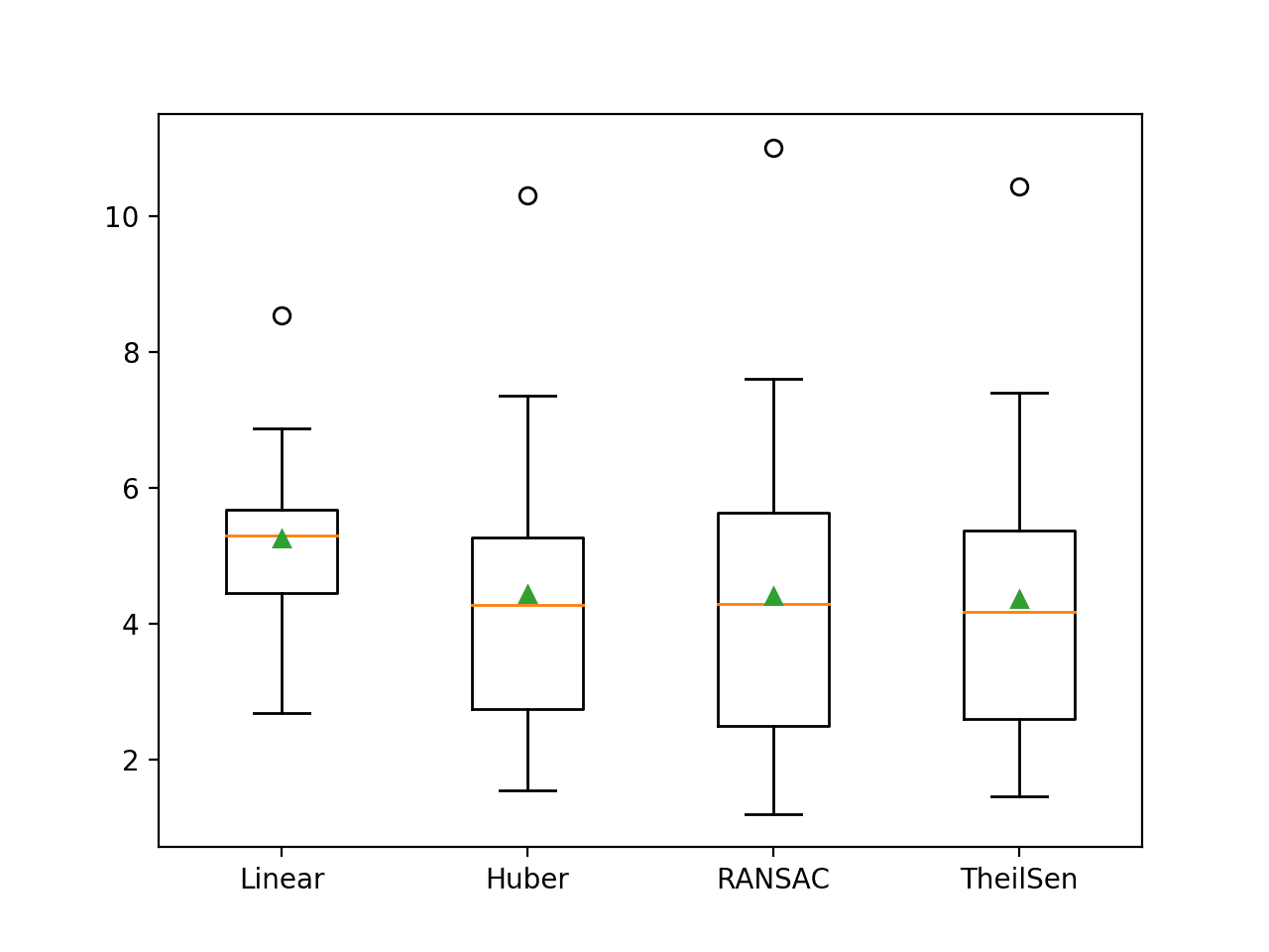
Nearest Shrunken Centroids With Python

$
0
0

Nearest Centroids is a linear classification machine learning algorithm.

It involves predicting a class label for new examples based on which class-based centroid the example is closest to from the training dataset.

The Nearest Shrunken Centroids algorithm is an extension that involves shifting class-based centroids toward the centroid of the entire training dataset and removing those input variables that are less useful at discriminating the classes.

As such, the Nearest Shrunken Centroids algorithm performs an automatic form of feature selection, making it appropriate for datasets with very large numbers of input variables.

In this tutorial, you will discover the Nearest Shrunken Centroids classification machine learning algorithm.

After completing this tutorial, you will know:

  • The Nearest Shrunken Centroids is a simple linear machine learning algorithm for classification.
  • How to fit, evaluate, and make predictions with the Nearest Shrunken Centroids model with Scikit-Learn.
  • How to tune the hyperparameters of the Nearest Shrunken Centroids algorithm on a given dataset.

Let’s get started.

Nearest Shrunken Centroids With Python

Nearest Shrunken Centroids With Python
Photo by Giuseppe Milo, some rights reserved.

Tutorial Overview

This tutorial is divided into three parts; they are:

  1. Nearest Centroids Algorithm
  2. Nearest Centroids With Scikit-Learn
  3. Tuning Nearest Centroid Hyperparameters

Nearest Centroids Algorithm

Nearest Centroids is a classification machine learning algorithm.

The algorithm involves first summarizing the training dataset into a set of centroids (centers), then using the centroids to make predictions for new examples.

For each class, the centroid of the data is found by taking the average value of each predictor (per class) in the training set. The overall centroid is computed using the data from all of the classes.

— Page 307, Applied Predictive Modeling, 2013.

A centroid is the geometric center of a data distribution, such as the mean. In multiple dimensions, this would be the mean value along each dimension, forming a point of center of the distribution across each variable.

The Nearest Centroids algorithm assumes that the centroids in the input feature space are different for each target label. The training data is split into groups by class label, then the centroid for each group of data is calculated. Each centroid is simply the mean value of each of the input variables. If there are two classes, then two centroids or points are calculated; three classes give three centroids, and so on.

The centroids then represent the “model.” Given new examples, such as those in the test set or new data, the distance between a given row of data and each centroid is calculated and the closest centroid is used to assign a class label to the example.

Distance measures, such as Euclidean distance, are used for numerical data or hamming distance for categorical data, in which case it is best practice to scale input variables via normalization or standardization prior to training the model. This is to ensure that input variables with large values don’t dominate the distance calculation.

An extension to the nearest centroid method for classification is to shrink the centroids of each input variable towards the centroid of the entire training dataset. Those variables that are shrunk down to the value of the data centroid can then be removed as they do not help to discriminate between the class labels.

As such, the amount of shrinkage applied to the centroids is a hyperparameter that can be tuned for the dataset and used to perform an automatic form of feature selection. Thus, it is appropriate for a dataset with a large number of input variables, some of which may be irrelevant or noisy.

Consequently, the nearest shrunken centroid model also conducts feature selection during the model training process.

— Page 307, Applied Predictive Modeling, 2013.

This approach is referred to as “Nearest Shrunken Centroids” and was first described by Robert Tibshirani, et al. in their 2002 paper titled “Diagnosis Of Multiple Cancer Types By Shrunken Centroids Of Gene Expression.”

Nearest Centroids With Scikit-Learn

The Nearest Shrunken Centroids is available in the scikit-learn Python machine learning library via the NearestCentroid class.

The class allows the configuration of the distance metric used in the algorithm via the “metric” argument, which defaults to ‘euclidean‘ for the Euclidean distance metric.

This can be changed to other built-in metrics such as ‘manhattan.’

...
# create the nearest centroid model
model = NearestCentroid(metric='euclidean')

By default, no shrinkage is used, but shrinkage can be specified via the “shrink_threshold” argument, which takes a floating point value between 0 and 1.

...
# create the nearest centroid model
model = NearestCentroid(metric='euclidean', shrink_threshold=0.5)

We can demonstrate the Nearest Shrunken Centroids with a worked example.

First, let’s define a synthetic classification dataset.

We will use the make_classification() function to create a dataset with 1,000 examples, each with 20 input variables.

The example creates and summarizes the dataset.

# test classification dataset
from sklearn.datasets import make_classification
# define dataset
X, y = make_classification(n_samples=1000, n_features=20, n_informative=15, n_redundant=5, random_state=1)
# summarize the dataset
print(X.shape, y.shape)

Running the example creates the dataset and confirms the number of rows and columns of the dataset.

(1000, 20) (1000,)

We can fit and evaluate a Nearest Shrunken Centroids model using repeated stratified k-fold cross-validation via the RepeatedStratifiedKFold class. We will use 10 folds and three repeats in the test harness.

We will use the default configuration of Euclidean distance and no shrinkage.

...
# create the nearest centroid model
model = NearestCentroid()

The complete example of evaluating the Nearest Shrunken Centroids model for the synthetic binary classification task is listed below.

# evaluate an nearest centroid model on the dataset
from numpy import mean
from numpy import std
from sklearn.datasets import make_classification
from sklearn.model_selection import cross_val_score
from sklearn.model_selection import RepeatedStratifiedKFold
from sklearn.neighbors import NearestCentroid
# define dataset
X, y = make_classification(n_samples=1000, n_features=20, n_informative=15, n_redundant=5, random_state=1)
# define model
model = NearestCentroid()
# define model evaluation method
cv = RepeatedStratifiedKFold(n_splits=10, n_repeats=3, random_state=1)
# evaluate model
scores = cross_val_score(model, X, y, scoring='accuracy', cv=cv, n_jobs=-1)
# summarize result
print('Mean Accuracy: %.3f (%.3f)' % (mean(scores), std(scores)))

Running the example evaluates the Nearest Shrunken Centroids algorithm on the synthetic dataset and reports the average accuracy across the three repeats of 10-fold cross-validation.

Your specific results may vary given the stochastic nature of the learning algorithm. Consider running the example a few times.

In this case, we can see that the model achieved a mean accuracy of about 71 percent.

Mean Accuracy: 0.711 (0.055)

We may decide to use the Nearest Shrunken Centroids as our final model and make predictions on new data.

This can be achieved by fitting the model on all available data and calling the predict() function passing in a new row of data.

We can demonstrate this with a complete example listed below.

# make a prediction with a nearest centroid model on the dataset
from sklearn.datasets import make_classification
from sklearn.neighbors import NearestCentroid
# define dataset
X, y = make_classification(n_samples=1000, n_features=20, n_informative=15, n_redundant=5, random_state=1)
# define model
model = NearestCentroid()
# fit model
model.fit(X, y)
# define new data
row = [2.47475454,0.40165523,1.68081787,2.88940715,0.91704519,-3.07950644,4.39961206,0.72464273,-4.86563631,-6.06338084,-1.22209949,-0.4699618,1.01222748,-0.6899355,-0.53000581,6.86966784,-3.27211075,-6.59044146,-2.21290585,-3.139579]
# make a prediction
yhat = model.predict([row])
# summarize prediction
print('Predicted Class: %d' % yhat)

Running the example fits the model and makes a class label prediction for a new row of data.

Predicted Class: 0

Next, we can look at configuring the model hyperparameters.

Tuning Nearest Centroid Hyperparameters

The hyperparameters for the Nearest Shrunken Centroid method must be configured for your specific dataset.

Perhaps the most important hyperparameter is the shrinkage controlled via the “shrink_threshold” argument. It is a good idea to test values between 0 and 1 on a grid of values such as 0.1 or 0.01.

The example below demonstrates this using the GridSearchCV class with a grid of values we have defined.

# grid search shrinkage for nearest centroid
from numpy import arange
from sklearn.datasets import make_classification
from sklearn.model_selection import GridSearchCV
from sklearn.model_selection import RepeatedStratifiedKFold
from sklearn.neighbors import NearestCentroid
# define dataset
X, y = make_classification(n_samples=1000, n_features=20, n_informative=15, n_redundant=5, random_state=1)
# define model
model = NearestCentroid()
# define model evaluation method
cv = RepeatedStratifiedKFold(n_splits=10, n_repeats=3, random_state=1)
# define grid
grid = dict()
grid['shrink_threshold'] = arange(0, 1.01, 0.01)
# define search
search = GridSearchCV(model, grid, scoring='accuracy', cv=cv, n_jobs=-1)
# perform the search
results = search.fit(X, y)
# summarize
print('Mean Accuracy: %.3f' % results.best_score_)
print('Config: %s' % results.best_params_)

Running the example will evaluate each combination of configurations using repeated cross-validation.

Your specific results may vary given the stochastic nature of the learning algorithm. Try running the example a few times.

In this case, we can see that we achieved slightly better results than the default, with 71.4 percent vs 71.1 percent. We can see that the model assigned a shrink_threshold value of 0.53.

Mean Accuracy: 0.714
Config: {'shrink_threshold': 0.53}

The other key configuration is the distance measure used, which can be chosen based on the distribution of the input variables.

Any of the built-in distance measures can be used, as listed here:

Common distance measures include:

  • ‘cityblock’, ‘cosine’, ‘euclidean’, ‘l1’, ‘l2’, ‘manhattan’

For more on how these distance measures are calculated, see the tutorial:

Given that our input variables are numeric, our dataset only supports ‘euclidean‘ and ‘manhattan.’

We can include these metrics in our grid search; the complete example is listed below.

# grid search shrinkage and distance metric for nearest centroid
from numpy import arange
from sklearn.datasets import make_classification
from sklearn.model_selection import GridSearchCV
from sklearn.model_selection import RepeatedStratifiedKFold
from sklearn.neighbors import NearestCentroid
# define dataset
X, y = make_classification(n_samples=1000, n_features=20, n_informative=15, n_redundant=5, random_state=1)
# define model
model = NearestCentroid()
# define model evaluation method
cv = RepeatedStratifiedKFold(n_splits=10, n_repeats=3, random_state=1)
# define grid
grid = dict()
grid['shrink_threshold'] = arange(0, 1.01, 0.01)
grid['metric'] = ['euclidean', 'manhattan']
# define search
search = GridSearchCV(model, grid, scoring='accuracy', cv=cv, n_jobs=-1)
# perform the search
results = search.fit(X, y)
# summarize
print('Mean Accuracy: %.3f' % results.best_score_)
print('Config: %s' % results.best_params_)

Running the example fits the model and discovers the hyperparameters that give the best results using cross-validation.

Your specific results may vary given the stochastic nature of the learning algorithm. Try running the example a few times.

In this case, we can see that we get slightly better accuracy of 75 percent using no shrinkage and the manhattan instead of the euclidean distance measure.

Mean Accuracy: 0.750
Config: {'metric': 'manhattan', 'shrink_threshold': 0.0}

A good extension to these experiments would be to add data normalization or standardization to the data as part of a modeling Pipeline.

Further Reading

This section provides more resources on the topic if you are looking to go deeper.

Tutorials

Papers

Books

APIs

Articles

Summary

In this tutorial, you discovered the Nearest Shrunken Centroids classification machine learning algorithm.

Specifically, you learned:

  • The Nearest Shrunken Centroids is a simple linear machine learning algorithm for classification.
  • How to fit, evaluate, and make predictions with the Nearest Shrunken Centroids model with Scikit-Learn.
  • How to tune the hyperparameters of the Nearest Shrunken Centroids algorithm on a given dataset.

Do you have any questions?
Ask your questions in the comments below and I will do my best to answer.

The post Nearest Shrunken Centroids With Python appeared first on Machine Learning Mastery.
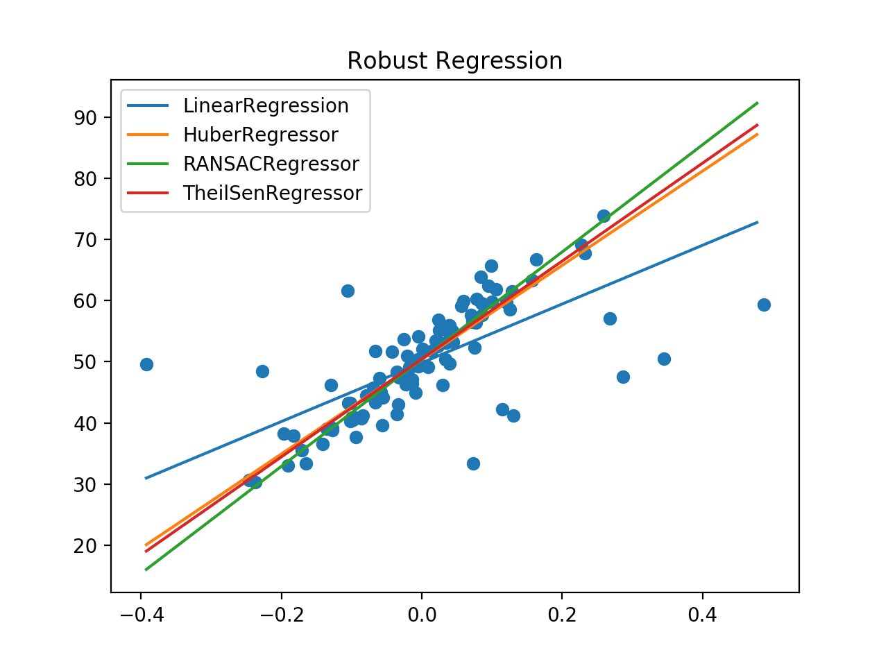
How to Develop LARS Regression Models in Python

$
0
0

Regression is a modeling task that involves predicting a numeric value given an input.

Linear regression is the standard algorithm for regression that assumes a linear relationship between inputs and the target variable. An extension to linear regression involves adding penalties to the loss function during training that encourage simpler models that have smaller coefficient values. These extensions are referred to as regularized linear regression or penalized linear regression.

Lasso Regression is a popular type of regularized linear regression that includes an L1 penalty. This has the effect of shrinking the coefficients for those input variables that do not contribute much to the prediction task.

Least Angle Regression or LARS for short provides an alternate, efficient way of fitting a Lasso regularized regression model that does not require any hyperparameters.

In this tutorial, you will discover how to develop and evaluate LARS Regression models in Python.

After completing this tutorial, you will know:

  • LARS Regression provides an alternate way to train a Lasso regularized linear regression model that adds a penalty to the loss function during training.
  • How to evaluate a LARS Regression model and use a final model to make predictions for new data.
  • How to configure the LARS Regression model for a new dataset automatically using a cross-validation version of the estimator.

Let’s get started.

How to Develop LARS Regression Models in Python

How to Develop LARS Regression Models in Python
Photo by Nicolas Raymond, some rights reserved.

Tutorial Overview

This tutorial is divided into three parts; they are:

  1. LARS Regression
  2. Example of LARS Regression
  3. Tuning LARS Hyperparameters

LARS Regression

Linear regression refers to a model that assumes a linear relationship between input variables and the target variable.

With a single input variable, this relationship is a line, and with higher dimensions, this relationship can be thought of as a hyperplane that connects the input variables to the target variable. The coefficients of the model are found via an optimization process that seeks to minimize the sum squared error between the predictions (yhat) and the expected target values (y).

  • loss = sum i=0 to n (y_i – yhat_i)^2

A problem with linear regression is that estimated coefficients of the model can become large, making the model sensitive to inputs and possibly unstable. This is particularly true for problems with few observations (samples) or more samples (n) than input predictors (p) or variables (so-called p >> n problems).

One approach to address the stability of regression models is to change the loss function to include additional costs for a model that has large coefficients. Linear regression models that use these modified loss functions during training are referred to collectively as penalized linear regression.

A popular penalty is to penalize a model based on the sum of the absolute coefficient values. This is called the L1 penalty. An L1 penalty minimizes the size of all coefficients and allows some coefficients to be minimized to the value zero, which removes the predictor from the model.

  • l1_penalty = sum j=0 to p abs(beta_j)

An L1 penalty minimizes the size of all coefficients and allows any coefficient to go to the value of zero, effectively removing input features from the model. This acts as a type of automatic feature selection method.

… a consequence of penalizing the absolute values is that some parameters are actually set to 0 for some value of lambda. Thus the lasso yields models that simultaneously use regularization to improve the model and to conduct feature selection.

— Page 125, Applied Predictive Modeling, 2013.

This penalty can be added to the cost function for linear regression and is referred to as Least Absolute Shrinkage And Selection Operator (LASSO), or more commonly, “Lasso” (with title case) for short.

The Lasso trains the model using a least-squares loss training procedure.

Least Angle Regression, LAR or LARS for short, is an alternative approach to solving the optimization problem of fitting the penalized model. Technically, LARS is a forward stepwise version of feature selection for regression that can be adapted for the Lasso model.

Unlike the Lasso, it does not require a hyperparameter that controls the weighting of the penalty in the loss function. Instead, the weighting is discovered automatically by LARS.

… least angle regression (LARS), is a broad framework that encompasses the lasso and similar models. The LARS model can be used to fit lasso models more efficiently, especially in high-dimensional problems.

— Page 126, Applied Predictive Modeling, 2013.

Now that we are familiar with LARS penalized regression, let’s look at a worked example.

Example of LARS Regression

In this section, we will demonstrate how to use the LARS Regression algorithm.

First, let’s introduce a standard regression dataset. We will use the housing dataset.

The housing dataset is a standard machine learning dataset comprising 506 rows of data with 13 numerical input variables and a numerical target variable.

Using a test harness of repeated stratified 10-fold cross-validation with three repeats, a naive model can achieve a mean absolute error (MAE) of about 6.6. A top-performing model can achieve a MAE on this same test harness of about 1.9. This provides the bounds of expected performance on this dataset.

The dataset involves predicting the house price given details of the house’s suburb in the American city of Boston.

No need to download the dataset; we will download it automatically as part of our worked examples.

The example below downloads and loads the dataset as a Pandas DataFrame and summarizes the shape of the dataset and the first five rows of data.

# load and summarize the housing dataset
from pandas import read_csv
from matplotlib import pyplot
# load dataset
url = 'https://raw.githubusercontent.com/jbrownlee/Datasets/master/housing.csv'
dataframe = read_csv(url, header=None)
# summarize shape
print(dataframe.shape)
# summarize first few lines
print(dataframe.head())

Running the example confirms the 506 rows of data and 13 input variables and a single numeric target variable (14 in total). We can also see that all input variables are numeric.

(506, 14)
        0     1     2   3      4      5   ...  8      9     10      11    12    13
0  0.00632  18.0  2.31   0  0.538  6.575  ...   1  296.0  15.3  396.90  4.98  24.0
1  0.02731   0.0  7.07   0  0.469  6.421  ...   2  242.0  17.8  396.90  9.14  21.6
2  0.02729   0.0  7.07   0  0.469  7.185  ...   2  242.0  17.8  392.83  4.03  34.7
3  0.03237   0.0  2.18   0  0.458  6.998  ...   3  222.0  18.7  394.63  2.94  33.4
4  0.06905   0.0  2.18   0  0.458  7.147  ...   3  222.0  18.7  396.90  5.33  36.2

[5 rows x 14 columns]

The scikit-learn Python machine learning library provides an implementation of the LARS penalized regression algorithm via the Lars class.

...
# define model
model = Lars()

We can evaluate the LARS Regression model on the housing dataset using repeated 10-fold cross-validation and report the average mean absolute error (MAE) on the dataset.

# evaluate an lars regression model on the dataset
from numpy import mean
from numpy import std
from numpy import absolute
from pandas import read_csv
from sklearn.model_selection import cross_val_score
from sklearn.model_selection import RepeatedKFold
from sklearn.linear_model import Lars
# load the dataset
url = 'https://raw.githubusercontent.com/jbrownlee/Datasets/master/housing.csv'
dataframe = read_csv(url, header=None)
data = dataframe.values
X, y = data[:, :-1], data[:, -1]
# define model
model = Lars()
# define model evaluation method
cv = RepeatedKFold(n_splits=10, n_repeats=3, random_state=1)
# evaluate model
scores = cross_val_score(model, X, y, scoring='neg_mean_absolute_error', cv=cv, n_jobs=-1)
# force scores to be positive
scores = absolute(scores)
print('Mean MAE: %.3f (%.3f)' % (mean(scores), std(scores)))

Running the example evaluates the LARS Regression algorithm on the housing dataset and reports the average MAE across the three repeats of 10-fold cross-validation.

Your specific results may vary given the stochastic nature of the learning algorithm. Consider running the example a few times.

In this case, we can see that the model achieved a MAE of about 3.432.

Mean MAE: 3.432 (0.552)

We may decide to use the LARS Regression as our final model and make predictions on new data.

This can be achieved by fitting the model on all available data and calling the predict() function, passing in a new row of data.

We can demonstrate this with a complete example, listed below.

# make a prediction with a lars regression model on the dataset
from pandas import read_csv
from sklearn.linear_model import Lars
# load the dataset
url = 'https://raw.githubusercontent.com/jbrownlee/Datasets/master/housing.csv'
dataframe = read_csv(url, header=None)
data = dataframe.values
X, y = data[:, :-1], data[:, -1]
# define model
model = Lars()
# fit model
model.fit(X, y)
# define new data
row = [0.00632,18.00,2.310,0,0.5380,6.5750,65.20,4.0900,1,296.0,15.30,396.90,4.98]
# make a prediction
yhat = model.predict([row])
# summarize prediction
print('Predicted: %.3f' % yhat)

Running the example fits the model and makes a prediction for the new rows of data.

Your specific results may vary given the stochastic nature of the learning algorithm. Try running the example a few times.

Predicted: 29.904

Next, we can look at configuring the model hyperparameters.

Tuning LARS Hyperparameters

As part of the LARS training algorithm, it automatically discovers the best value for the lambda hyperparameter used in the Lasso algorithm.

This hyperparameter is referred to as the “alpha” argument in the scikit-learn implementation of Lasso and LARS.

Nevertheless, the process of automatically discovering the best model and alpha hyperparameter is still based on a single training dataset.

An alternative approach is to fit the model on multiple subsets of the training dataset and choose the best internal model configuration across the folds, in this case, the value of alpha. Generally, this is referred to as a cross-validation estimator.

The scikit-learn libraries offer a cross-validation version of the LARS for finding a more robust value for alpha via the LarsCV class.

The example below demonstrates how to fit a LarsCV model and report the alpha value found via cross-validation

# use automatically configured the lars regression algorithm
from numpy import arange
from pandas import read_csv
from sklearn.linear_model import LarsCV
from sklearn.model_selection import RepeatedKFold
# load the dataset
url = 'https://raw.githubusercontent.com/jbrownlee/Datasets/master/housing.csv'
dataframe = read_csv(url, header=None)
data = dataframe.values
X, y = data[:, :-1], data[:, -1]
# define model evaluation method
cv = RepeatedKFold(n_splits=10, n_repeats=3, random_state=1)
# define model
model = LarsCV(cv=cv, n_jobs=-1)
# fit model
model.fit(X, y)
# summarize chosen configuration
print('alpha: %f' % model.alpha_)

Running the example fits the LarsCV model using repeated cross-validation and reports an optimal alpha value found across the runs.

alpha: 0.001623

This version of the LARS model may prove more robust in practice.

We can evaluate it using the same procedure we did in the previous section, although in this case, each model fit is based on the hyperparameters found via repeated k-fold cross-validation internally (e.g. cross-validation of a cross-validation estimator).

The complete example is listed below.

# evaluate an lars cross-validation regression model on the dataset
from numpy import mean
from numpy import std
from numpy import absolute
from pandas import read_csv
from sklearn.model_selection import cross_val_score
from sklearn.model_selection import RepeatedKFold
from sklearn.linear_model import LarsCV
# load the dataset
url = 'https://raw.githubusercontent.com/jbrownlee/Datasets/master/housing.csv'
dataframe = read_csv(url, header=None)
data = dataframe.values
X, y = data[:, :-1], data[:, -1]
# define model evaluation method
cv = RepeatedKFold(n_splits=10, n_repeats=3, random_state=1)
# define model
model = LarsCV(cv=cv, n_jobs=-1)
# evaluate model
scores = cross_val_score(model, X, y, scoring='neg_mean_absolute_error', cv=cv, n_jobs=-1)
# force scores to be positive
scores = absolute(scores)
print('Mean MAE: %.3f (%.3f)' % (mean(scores), std(scores)))

Running the example will evaluate the cross-validated estimation of model hyperparameters using repeated cross-validation.

Your specific results may vary given the stochastic nature of the learning algorithm. Try running the example a few times.

In this case, we can see that we achieved slightly better results with 3.374 vs. 3.432 in the previous section.

Mean MAE: 3.374 (0.558)

Further Reading

This section provides more resources on the topic if you are looking to go deeper.

Books

APIs

Articles

Summary

In this tutorial, you discovered how to develop and evaluate LARS Regression models in Python.

Specifically, you learned:

  • LARS Regression provides an alternate way to train a Lasso regularized linear regression model that adds a penalty to the loss function during training.
  • How to evaluate a LARS Regression model and use a final model to make predictions for new data.
  • How to configure the LARS Regression model for a new dataset automatically using a cross-validation version of the estimator.

Do you have any questions?
Ask your questions in the comments below and I will do my best to answer.

The post How to Develop LARS Regression Models in Python appeared first on Machine Learning Mastery.


How to Identify Overfitting Machine Learning Models in Scikit-Learn

$
0
0

Overfitting is a common explanation for the poor performance of a predictive model.

An analysis of learning dynamics can help to identify whether a model has overfit the training dataset and may suggest an alternate configuration to use that could result in better predictive performance.

Performing an analysis of learning dynamics is straightforward for algorithms that learn incrementally, like neural networks, but it is less clear how we might perform the same analysis with other algorithms that do not learn incrementally, such as decision trees, k-nearest neighbors, and other general algorithms in the scikit-learn machine learning library.

In this tutorial, you will discover how to identify overfitting for machine learning models in Python.

After completing this tutorial, you will know:

  • Overfitting is a possible cause of poor generalization performance of a predictive model.
  • Overfitting can be analyzed for machine learning models by varying key model hyperparameters.
  • Although overfitting is a useful tool for analysis, it must not be confused with model selection.

Let’s get started.

Identify Overfitting Machine Learning Models With Scikit-Learn

Identify Overfitting Machine Learning Models With Scikit-Learn
Photo by Bonnie Moreland, some rights reserved.

Tutorial Overview

This tutorial is divided into five parts; they are:

  1. What Is Overfitting
  2. How to Perform an Overfitting Analysis
  3. Example of Overfitting in Scikit-Learn
  4. Counterexample of Overfitting in Scikit-Learn
  5. Separate Overfitting Analysis From Model Selection

What Is Overfitting

Overfitting refers to an unwanted behavior of a machine learning algorithm used for predictive modeling.

It is the case where model performance on the training dataset is improved at the cost of worse performance on data not seen during training, such as a holdout test dataset or new data.

We can identify if a machine learning model has overfit by first evaluating the model on the training dataset and then evaluating the same model on a holdout test dataset.

If the performance of the model on the training dataset is significantly better than the performance on the test dataset, then the model may have overfit the training dataset.

We care about overfitting because it is a common cause for “poor generalization” of the model as measured by high “generalization error.” That is error made by the model when making predictions on new data.

This means, if our model has poor performance, maybe it is because it has overfit.

But what does it mean if a model’s performance is “significantly better” on the training set compared to the test set?

For example, it is common and perhaps normal for the model to have better performance on the training set than the test set.

As such, we can perform an analysis of the algorithm on the dataset to better expose the overfitting behavior.

How to Perform an Overfitting Analysis

An overfitting analysis is an approach for exploring how and when a specific model is overfitting on a specific dataset.

It is a tool that can help you learn more about the learning dynamics of a machine learning model.

This might be achieved by reviewing the model behavior during a single run for algorithms like neural networks that are fit on the training dataset incrementally.

A plot of the model performance on the train and test set can be calculated at each point during training and plots can be created. This plot is often called a learning curve plot, showing one curve for model performance on the training set and one curve for the test set for each increment of learning.

If you would like to learn more about learning curves for algorithms that learn incrementally, see the tutorial:

The common pattern for overfitting can be seen on learning curve plots, where model performance on the training dataset continues to improve (e.g. loss or error continues to fall or accuracy continues to rise) and performance on the test or validation set improves to a point and then begins to get worse.

If this pattern is observed, then training should stop at that point where performance gets worse on the test or validation set for algorithms that learn incrementally

This makes sense for algorithms that learn incrementally like neural networks, but what about other algorithms?

  • How do you perform an overfitting analysis for machine learning algorithms in scikit-learn?

One approach for performing an overfitting analysis on algorithms that do not learn incrementally is by varying a key model hyperparameter and evaluating the model performance on the train and test sets for each configuration.

To make this clear, let’s explore a case of analyzing a model for overfitting in the next section.

Example of Overfitting in Scikit-Learn

In this section, we will look at an example of overfitting a machine learning model to a training dataset.

First, let’s define a synthetic classification dataset.

We will use the make_classification() function to define a binary (two class) classification prediction problem with 10,000 examples (rows) and 20 input features (columns).

The example below creates the dataset and summarizes the shape of the input and output components.

# synthetic classification dataset
from sklearn.datasets import make_classification
# define dataset
X, y = make_classification(n_samples=10000, n_features=20, n_informative=5, n_redundant=15, random_state=1)
# summarize the dataset
print(X.shape, y.shape)

Running the example creates the dataset and reports the shape, confirming our expectations.

(10000, 20) (10000,)

Next, we need to split the dataset into train and test subsets.

We will use the train_test_split() function and split the data into 70 percent for training a model and 30 percent for evaluating it.

# split a dataset into train and test sets
from sklearn.datasets import make_classification
from sklearn.model_selection import train_test_split
# create dataset
X, y = make_classification(n_samples=10000, n_features=20, n_informative=5, n_redundant=15, random_state=1)
# split into train test sets
X_train, X_test, y_train, y_test = train_test_split(X, y, test_size=0.3)
# summarize the shape of the train and test sets
print(X_train.shape, X_test.shape, y_train.shape, y_test.shape)

Running the example splits the dataset and we can confirm that we have 70k examples for training and 30k for evaluating a model.

(7000, 20) (3000, 20) (7000,) (3000,)

Next, we can explore a machine learning model overfitting the training dataset.

We will use a decision tree via the DecisionTreeClassifier and test different tree depths with the “max_depth” argument.

Shallow decision trees (e.g. few levels) generally do not overfit but have poor performance (high bias, low variance). Whereas deep trees (e.g. many levels) generally do overfit and have good performance (low bias, high variance). A desirable tree is one that is not so shallow that it has low skill and not so deep that it overfits the training dataset.

We evaluate decision tree depths from 1 to 20.

...
# define the tree depths to evaluate
values = [i for i in range(1, 21)]

We will enumerate each tree depth, fit a tree with a given depth on the training dataset, then evaluate the tree on both the train and test sets.

The expectation is that as the depth of the tree increases, performance on train and test will improve to a point, and as the tree gets too deep, it will begin to overfit the training dataset at the expense of worse performance on the holdout test set.

...
# evaluate a decision tree for each depth
for i in values:
	# configure the model
	model = DecisionTreeClassifier(max_depth=i)
	# fit model on the training dataset
	model.fit(X_train, y_train)
	# evaluate on the train dataset
	train_yhat = model.predict(X_train)
	train_acc = accuracy_score(y_train, train_yhat)
	train_scores.append(train_acc)
	# evaluate on the test dataset
	test_yhat = model.predict(X_test)
	test_acc = accuracy_score(y_test, test_yhat)
	test_scores.append(test_acc)
	# summarize progress
	print('>%d, train: %.3f, test: %.3f' % (i, train_acc, test_acc))

At the end of the run, we will then plot all model accuracy scores on the train and test sets for visual comparison.

...
# plot of train and test scores vs tree depth
pyplot.plot(values, train_scores, '-o', label='Train')
pyplot.plot(values, test_scores, '-o', label='Test')
pyplot.legend()
pyplot.show()

Tying this together, the complete example of exploring different tree depths on the synthetic binary classification dataset is listed below.

# evaluate decision tree performance on train and test sets with different tree depths
from sklearn.datasets import make_classification
from sklearn.model_selection import train_test_split
from sklearn.metrics import accuracy_score
from sklearn.tree import DecisionTreeClassifier
from matplotlib import pyplot
# create dataset
X, y = make_classification(n_samples=10000, n_features=20, n_informative=5, n_redundant=15, random_state=1)
# split into train test sets
X_train, X_test, y_train, y_test = train_test_split(X, y, test_size=0.3)
# define lists to collect scores
train_scores, test_scores = list(), list()
# define the tree depths to evaluate
values = [i for i in range(1, 21)]
# evaluate a decision tree for each depth
for i in values:
	# configure the model
	model = DecisionTreeClassifier(max_depth=i)
	# fit model on the training dataset
	model.fit(X_train, y_train)
	# evaluate on the train dataset
	train_yhat = model.predict(X_train)
	train_acc = accuracy_score(y_train, train_yhat)
	train_scores.append(train_acc)
	# evaluate on the test dataset
	test_yhat = model.predict(X_test)
	test_acc = accuracy_score(y_test, test_yhat)
	test_scores.append(test_acc)
	# summarize progress
	print('>%d, train: %.3f, test: %.3f' % (i, train_acc, test_acc))
# plot of train and test scores vs tree depth
pyplot.plot(values, train_scores, '-o', label='Train')
pyplot.plot(values, test_scores, '-o', label='Test')
pyplot.legend()
pyplot.show()

Running the example fits and evaluates a decision tree on the train and test sets for each tree depth and reports the accuracy scores.

Note: Your results may vary given the stochastic nature of the algorithm or evaluation procedure, or differences in numerical precision. Consider running the example a few times and compare the average outcome.

In this case, we can see a trend of increasing accuracy on the training dataset with the tree depth to a point around a depth of 19-20 levels where the tree fits the training dataset perfectly.

We can also see that the accuracy on the test set improves with tree depth until a depth of about eight or nine levels, after which accuracy begins to get worse with each increase in tree depth.

This is exactly what we would expect to see in a pattern of overfitting.

We would choose a tree depth of eight or nine before the model begins to overfit the training dataset.

>1, train: 0.769, test: 0.761
>2, train: 0.808, test: 0.804
>3, train: 0.879, test: 0.878
>4, train: 0.902, test: 0.896
>5, train: 0.915, test: 0.903
>6, train: 0.929, test: 0.918
>7, train: 0.942, test: 0.921
>8, train: 0.951, test: 0.924
>9, train: 0.959, test: 0.926
>10, train: 0.968, test: 0.923
>11, train: 0.977, test: 0.925
>12, train: 0.983, test: 0.925
>13, train: 0.987, test: 0.926
>14, train: 0.992, test: 0.921
>15, train: 0.995, test: 0.920
>16, train: 0.997, test: 0.913
>17, train: 0.999, test: 0.918
>18, train: 0.999, test: 0.918
>19, train: 1.000, test: 0.914
>20, train: 1.000, test: 0.913

A figure is also created that shows line plots of the model accuracy on the train and test sets with different tree depths.

The plot clearly shows that increasing the tree depth in the early stages results in a corresponding improvement in both train and test sets.

This continues until a depth of around 10 levels, after which the model is shown to overfit the training dataset at the cost of worse performance on the holdout dataset.

Line Plot of Decision Tree Accuracy on Train and Test Datasets for Different Tree Depths

Line Plot of Decision Tree Accuracy on Train and Test Datasets for Different Tree Depths

This analysis is interesting. It shows why the model has a worse hold-out test set performance when “max_depth” is set to large values.

But it is not required.

We can just as easily choose a “max_depth” using a grid search without performing an analysis on why some values result in better performance and some result in worse performance.

In fact, in the next section, we will show where this analysis can be misleading.

Counterexample of Overfitting in Scikit-Learn

Sometimes, we may perform an analysis of machine learning model behavior and be deceived by the results.

A good example of this is varying the number of neighbors for the k-nearest neighbors algorithms, which we can implement using the KNeighborsClassifier class and configure via the “n_neighbors” argument.

Let’s forget how KNN works for the moment.

We can perform the same analysis of the KNN algorithm as we did in the previous section for the decision tree and see if our model overfits for different configuration values. In this case, we will vary the number of neighbors from 1 to 50 to get more of the effect.

The complete example is listed below.

# evaluate knn performance on train and test sets with different numbers of neighbors
from sklearn.datasets import make_classification
from sklearn.model_selection import train_test_split
from sklearn.metrics import accuracy_score
from sklearn.neighbors import KNeighborsClassifier
from matplotlib import pyplot
# create dataset
X, y = make_classification(n_samples=10000, n_features=20, n_informative=5, n_redundant=15, random_state=1)
# split into train test sets
X_train, X_test, y_train, y_test = train_test_split(X, y, test_size=0.3)
# define lists to collect scores
train_scores, test_scores = list(), list()
# define the tree depths to evaluate
values = [i for i in range(1, 51)]
# evaluate a decision tree for each depth
for i in values:
	# configure the model
	model = KNeighborsClassifier(n_neighbors=i)
	# fit model on the training dataset
	model.fit(X_train, y_train)
	# evaluate on the train dataset
	train_yhat = model.predict(X_train)
	train_acc = accuracy_score(y_train, train_yhat)
	train_scores.append(train_acc)
	# evaluate on the test dataset
	test_yhat = model.predict(X_test)
	test_acc = accuracy_score(y_test, test_yhat)
	test_scores.append(test_acc)
	# summarize progress
	print('>%d, train: %.3f, test: %.3f' % (i, train_acc, test_acc))
# plot of train and test scores vs number of neighbors
pyplot.plot(values, train_scores, '-o', label='Train')
pyplot.plot(values, test_scores, '-o', label='Test')
pyplot.legend()
pyplot.show()

Running the example fits and evaluates a KNN model on the train and test sets for each number of neighbors and reports the accuracy scores.

Note: Your results may vary given the stochastic nature of the algorithm or evaluation procedure, or differences in numerical precision. Consider running the example a few times and compare the average outcome.

Recall, we are looking for a pattern where performance on the test set improves and then starts to get worse, and performance on the training set continues to improve.

We do not see this pattern.

Instead, we see that accuracy on the training dataset starts at perfect accuracy and falls with almost every increase in the number of neighbors.

We also see that performance of the model on the holdout test improves to a value of about five neighbors, holds level and begins a downward trend after that.

>1, train: 1.000, test: 0.919
>2, train: 0.965, test: 0.916
>3, train: 0.962, test: 0.932
>4, train: 0.957, test: 0.932
>5, train: 0.954, test: 0.935
>6, train: 0.953, test: 0.934
>7, train: 0.952, test: 0.932
>8, train: 0.951, test: 0.933
>9, train: 0.949, test: 0.933
>10, train: 0.950, test: 0.935
>11, train: 0.947, test: 0.934
>12, train: 0.947, test: 0.933
>13, train: 0.945, test: 0.932
>14, train: 0.945, test: 0.932
>15, train: 0.944, test: 0.932
>16, train: 0.944, test: 0.934
>17, train: 0.943, test: 0.932
>18, train: 0.943, test: 0.935
>19, train: 0.942, test: 0.933
>20, train: 0.943, test: 0.935
>21, train: 0.942, test: 0.933
>22, train: 0.943, test: 0.933
>23, train: 0.941, test: 0.932
>24, train: 0.942, test: 0.932
>25, train: 0.942, test: 0.931
>26, train: 0.941, test: 0.930
>27, train: 0.941, test: 0.932
>28, train: 0.939, test: 0.932
>29, train: 0.938, test: 0.931
>30, train: 0.938, test: 0.931
>31, train: 0.937, test: 0.931
>32, train: 0.938, test: 0.931
>33, train: 0.937, test: 0.930
>34, train: 0.938, test: 0.931
>35, train: 0.937, test: 0.930
>36, train: 0.937, test: 0.928
>37, train: 0.936, test: 0.930
>38, train: 0.937, test: 0.930
>39, train: 0.935, test: 0.929
>40, train: 0.936, test: 0.929
>41, train: 0.936, test: 0.928
>42, train: 0.936, test: 0.929
>43, train: 0.936, test: 0.930
>44, train: 0.935, test: 0.929
>45, train: 0.935, test: 0.929
>46, train: 0.934, test: 0.929
>47, train: 0.935, test: 0.929
>48, train: 0.934, test: 0.929
>49, train: 0.934, test: 0.929
>50, train: 0.934, test: 0.929

A figure is also created that shows line plots of the model accuracy on the train and test sets with different numbers of neighbors.

The plots make the situation clearer. It looks as though the line plot for the training set is dropping to converge with the line for the test set. Indeed, this is exactly what is happening.

Line Plot of KNN Accuracy on Train and Test Datasets for Different Numbers of Neighbors

Line Plot of KNN Accuracy on Train and Test Datasets for Different Numbers of Neighbors

Now, recall how KNN works.

The “model” is really just the entire training dataset stored in an efficient data structure. Skill for the “model” on the training dataset should be 100 percent and anything less is unforgivable.

In fact, this argument holds for any machine learning algorithm and slices to the core of the confusion around overfitting for beginners.

Separate Overfitting Analysis From Model Selection

Overfitting can be an explanation for poor performance of a predictive model.

Creating learning curve plots that show the learning dynamics of a model on the train and test dataset is a helpful analysis for learning more about a model on a dataset.

But overfitting should not be confused with model selection.

We choose a predictive model or model configuration based on its out-of-sample performance. That is, its performance on new data not seen during training.

The reason we do this is that in predictive modeling, we are primarily interested in a model that makes skillful predictions. We want the model that can make the best possible predictions given the time and computational resources we have available.

This might mean we choose a model that looks like it has overfit the training dataset. In which case, an overfit analysis might be misleading.

It might also mean that the model has poor or terrible performance on the training dataset.

In general, if we cared about model performance on the training dataset in model selection, then we would expect a model to have perfect performance on the training dataset. It’s data we have available; we should not tolerate anything less.

As we saw with the KNN example above, we can achieve perfect performance on the training set by storing the training set directly and returning predictions with one neighbor at the cost of poor performance on any new data.

  • Wouldn’t a model that performs well on both train and test datasets be a better model?

Maybe. But, maybe not.

This argument is based on the idea that a model that performs well on both train and test sets has a better understanding of the underlying problem.

A corollary is that a model that performs well on the test set but poor on the training set is lucky (e.g. a statistical fluke) and a model that performs well on the train set but poor on the test set is overfit.

I believe this is the sticking point for beginners that often ask how to fix overfitting for their scikit-learn machine learning model.

The worry is that a model must perform well on both train and test sets, otherwise, they are in trouble.

This is not the case.

Performance on the training set is not relevant during model selection. You must focus on the out-of-sample performance only when choosing a predictive model.

Further Reading

This section provides more resources on the topic if you are looking to go deeper.

Tutorials

APIs

Articles

Summary

In this tutorial, you discovered how to identify overfitting for machine learning models in Python.

Specifically, you learned:

  • Overfitting is a possible cause of poor generalization performance of a predictive model.
  • Overfitting can be analyzed for machine learning models by varying key model hyperparameters.
  • Although overfitting is a useful tool for analysis, it must not be confused with model selection.

Do you have any questions?
Ask your questions in the comments below and I will do my best to answer.

The post How to Identify Overfitting Machine Learning Models in Scikit-Learn appeared first on Machine Learning Mastery.

A Gentle Introduction to PyCaret for Machine Learning

$
0
0

PyCaret is a Python open source machine learning library designed to make performing standard tasks in a machine learning project easy.

It is a Python version of the Caret machine learning package in R, popular because it allows models to be evaluated, compared, and tuned on a given dataset with just a few lines of code.

The PyCaret library provides these features, allowing the machine learning practitioner in Python to spot check a suite of standard machine learning algorithms on a classification or regression dataset with a single function call.

In this tutorial, you will discover the PyCaret Python open source library for machine learning.

After completing this tutorial, you will know:

  • PyCaret is a Python version of the popular and widely used caret machine learning package in R.
  • How to use PyCaret to easily evaluate and compare standard machine learning models on a dataset.
  • How to use PyCaret to easily tune the hyperparameters of a well-performing machine learning model.

Let’s get started.

A Gentle Introduction to PyCaret for Machine Learning

A Gentle Introduction to PyCaret for Machine Learning
Photo by Thomas, some rights reserved.

Tutorial Overview

This tutorial is divided into four parts; they are:

  1. What Is PyCaret?
  2. Sonar Dataset
  3. Comparing Machine Learning Models
  4. Tuning Machine Learning Models

What Is PyCaret?

PyCaret is an open source Python machine learning library inspired by the caret R package.

The goal of the caret package is to automate the major steps for evaluating and comparing machine learning algorithms for classification and regression. The main benefit of the library is that a lot can be achieved with very few lines of code and little manual configuration. The PyCaret library brings these capabilities to Python.

PyCaret is an open-source, low-code machine learning library in Python that aims to reduce the cycle time from hypothesis to insights. It is well suited for seasoned data scientists who want to increase the productivity of their ML experiments by using PyCaret in their workflows or for citizen data scientists and those new to data science with little or no background in coding.

PyCaret Homepage

The PyCaret library automates many steps of a machine learning project, such as:

  • Defining the data transforms to perform (setup())
  • Evaluating and comparing standard models (compare_models())
  • Tuning model hyperparameters (tune_model())

As well as many more features not limited to creating ensembles, saving models, and deploying models.

The PyCaret library has a wealth of documentation for using the API; you can get started here:

We will not explore all of the features of the library in this tutorial; instead, we will focus on simple machine learning model comparison and hyperparameter tuning.

You can install PyCaret using your Python package manager, such as pip. For example:

pip install pycaret

Once installed, we can confirm that the library is available in your development environment and is working correctly by printing the installed version.

# check pycaret version
import pycaret
print('PyCaret: %s' % pycaret.__version__)

Running the example will load the PyCaret library and print the installed version number.

Your version number should be the same or higher.

PyCaret: 2.0.0

If you need help installing PyCaret for your system, you can see the installation instructions here:

Now that we are familiar with what PyCaret is, let’s explore how we might use it on a machine learning project.

Sonar Dataset

We will use the Sonar standard binary classification dataset. You can learn more about it here:

We can download the dataset directly from the URL and load it as a Pandas DataFrame.

...
# define the location of the dataset
url = 'https://raw.githubusercontent.com/jbrownlee/Datasets/master/sonar.csv'
# load the dataset
df = read_csv(url, header=None)
# summarize the shape of the dataset
print(df.shape)

The PyCaret seems to require that a dataset has column names, and our dataset does not have column names, so we can set the column number as the column name directly.

...
# set column names as the column number
n_cols = df.shape[1]
df.columns = [str(i) for i in range(n_cols)]

Finally, we can summarize the first few rows of data.

...
# summarize the first few rows of data
print(df.head())

Tying this together, the complete example of loading and summarizing the Sonar dataset is listed below.

# load the sonar dataset
from pandas import read_csv
# define the location of the dataset
url = 'https://raw.githubusercontent.com/jbrownlee/Datasets/master/sonar.csv'
# load the dataset
df = read_csv(url, header=None)
# summarize the shape of the dataset
print(df.shape)
# set column names as the column number
n_cols = df.shape[1]
df.columns = [str(i) for i in range(n_cols)]
# summarize the first few rows of data
print(df.head())

Running the example first loads the dataset and reports the shape, showing it has 208 rows and 61 columns.

The first five rows are then printed showing that the input variables are all numeric and the target variable is column “60” and has string labels.

(208, 61)
0 1 2 3 4 ... 56 57 58 59 60
0 0.0200 0.0371 0.0428 0.0207 0.0954 ... 0.0180 0.0084 0.0090 0.0032 R
1 0.0453 0.0523 0.0843 0.0689 0.1183 ... 0.0140 0.0049 0.0052 0.0044 R
2 0.0262 0.0582 0.1099 0.1083 0.0974 ... 0.0316 0.0164 0.0095 0.0078 R
3 0.0100 0.0171 0.0623 0.0205 0.0205 ... 0.0050 0.0044 0.0040 0.0117 R
4 0.0762 0.0666 0.0481 0.0394 0.0590 ... 0.0072 0.0048 0.0107 0.0094 R

Next, we can use PyCaret to evaluate and compare a suite of standard machine learning algorithms to quickly discover what works well on this dataset.

PyCaret for Comparing Machine Learning Models

In this section, we will evaluate and compare the performance of standard machine learning models on the Sonar classification dataset.

First, we must set the dataset with the PyCaret library via the setup() function. This requires that we provide the Pandas DataFrame and specify the name of the column that contains the target variable.

The setup() function also allows you to configure simple data preparation, such as scaling, power transforms, missing data handling, and PCA transforms.

We will specify the data, target variable, and turn off HTML output, verbose output, and requests for user feedback.

...
# setup the dataset
grid = setup(data=df, target=df.columns[-1], html=False, silent=True, verbose=False)

Next, we can compare standard machine learning models by calling the compare_models() function.

By default, it will evaluate models using 10-fold cross-validation, sort results by classification accuracy, and return the single best model.

These are good defaults, and we don’t need to change a thing.

...
# evaluate models and compare models
best = compare_models()

Call the compare_models() function will also report a table of results summarizing all of the models that were evaluated and their performance.

Finally, we can report the best-performing model and its configuration.

Tying this together, the complete example of evaluating a suite of standard models on the Sonar classification dataset is listed below.

# compare machine learning algorithms on the sonar classification dataset
from pandas import read_csv
from pycaret.classification import setup
from pycaret.classification import compare_models
# define the location of the dataset
url = 'https://raw.githubusercontent.com/jbrownlee/Datasets/master/sonar.csv'
# load the dataset
df = read_csv(url, header=None)
# set column names as the column number
n_cols = df.shape[1]
df.columns = [str(i) for i in range(n_cols)]
# setup the dataset
grid = setup(data=df, target=df.columns[-1], html=False, silent=True, verbose=False)
# evaluate models and compare models
best = compare_models()
# report the best model
print(best)

Running the example will load the dataset, configure the PyCaret library, evaluate a suite of standard models, and report the best model found for the dataset.

Note: Your results may vary given the stochastic nature of the algorithm or evaluation procedure, or differences in numerical precision. Consider running the example a few times and compare the average outcome.

In this case, we can see that the “Extra Trees Classifier” has the best accuracy on the dataset with a score of about 86.95 percent.

We can then see the configuration of the model that was used, which looks like it used default hyperparameter values.

Model  Accuracy     AUC  Recall   Prec.      F1  \
0            Extra Trees Classifier    0.8695  0.9497  0.8571  0.8778  0.8631
1               CatBoost Classifier    0.8695  0.9548  0.8143  0.9177  0.8508
2   Light Gradient Boosting Machine    0.8219  0.9096  0.8000  0.8327  0.8012
3      Gradient Boosting Classifier    0.8010  0.8801  0.7690  0.8110  0.7805
4              Ada Boost Classifier    0.8000  0.8474  0.7952  0.8071  0.7890
5            K Neighbors Classifier    0.7995  0.8613  0.7405  0.8276  0.7773
6         Extreme Gradient Boosting    0.7995  0.8934  0.7833  0.8095  0.7802
7          Random Forest Classifier    0.7662  0.8778  0.6976  0.8024  0.7345
8          Decision Tree Classifier    0.7533  0.7524  0.7119  0.7655  0.7213
9                  Ridge Classifier    0.7448  0.0000  0.6952  0.7574  0.7135
10                      Naive Bayes    0.7214  0.8159  0.8286  0.6700  0.7308
11              SVM - Linear Kernel    0.7181  0.0000  0.6286  0.7146  0.6309
12              Logistic Regression    0.7100  0.8104  0.6357  0.7263  0.6634
13     Linear Discriminant Analysis    0.6924  0.7510  0.6667  0.6762  0.6628
14  Quadratic Discriminant Analysis    0.5800  0.6308  0.1095  0.5000  0.1750

     Kappa     MCC  TT (Sec)
0   0.7383  0.7446    0.1415
1   0.7368  0.7552    1.9930
2   0.6410  0.6581    0.0134
3   0.5989  0.6090    0.1413
4   0.5979  0.6123    0.0726
5   0.5957  0.6038    0.0019
6   0.5970  0.6132    0.0287
7   0.5277  0.5438    0.1107
8   0.5028  0.5192    0.0035
9   0.4870  0.5003    0.0030
10  0.4488  0.4752    0.0019
11  0.4235  0.4609    0.0024
12  0.4143  0.4285    0.0059
13  0.3825  0.3927    0.0034
14  0.1172  0.1792    0.0033
ExtraTreesClassifier(bootstrap=False, ccp_alpha=0.0, class_weight=None,
                     criterion='gini', max_depth=None, max_features='auto',
                     max_leaf_nodes=None, max_samples=None,
                     min_impurity_decrease=0.0, min_impurity_split=None,
                     min_samples_leaf=1, min_samples_split=2,
                     min_weight_fraction_leaf=0.0, n_estimators=100, n_jobs=-1,
                     oob_score=False, random_state=2728, verbose=0,
                     warm_start=False)

We could use this configuration directly and fit a model on the entire dataset and use it to make predictions on new data.

We can also use the table of results to get an idea of the types of models that perform well on the dataset, in this case, ensembles of decision trees.

Now that we are familiar with how to compare machine learning models using PyCaret, let’s look at how we might use the library to tune model hyperparameters.

Tuning Machine Learning Models

In this section, we will tune the hyperparameters of a machine learning model on the Sonar classification dataset.

We must load and set up the dataset as we did before when comparing models.

...
# setup the dataset
grid = setup(data=df, target=df.columns[-1], html=False, silent=True, verbose=False)

We can tune model hyperparameters using the tune_model() function in the PyCaret library.

The function takes an instance of the model to tune as input and knows what hyperparameters to tune automatically. A random search of model hyperparameters is performed and the total number of evaluations can be controlled via the “n_iter” argument.

By default, the function will optimize the ‘Accuracy‘ and will evaluate the performance of each configuration using 10-fold cross-validation, although this sensible default configuration can be changed.

We can perform a random search of the extra trees classifier as follows:

...
# tune model hyperparameters
best = tune_model(ExtraTreesClassifier(), n_iter=200)

The function will return the best-performing model, which can be used directly or printed to determine the hyperparameters that were selected.

It will also print a table of the results for the best configuration across the number of folds in the k-fold cross-validation (e.g. 10 folds).

Tying this together, the complete example of tuning the hyperparameters of the extra trees classifier on the Sonar dataset is listed below.

# tune model hyperparameters on the sonar classification dataset
from pandas import read_csv
from sklearn.ensemble import ExtraTreesClassifier
from pycaret.classification import setup
from pycaret.classification import tune_model
# define the location of the dataset
url = 'https://raw.githubusercontent.com/jbrownlee/Datasets/master/sonar.csv'
# load the dataset
df = read_csv(url, header=None)
# set column names as the column number
n_cols = df.shape[1]
df.columns = [str(i) for i in range(n_cols)]
# setup the dataset
grid = setup(data=df, target=df.columns[-1], html=False, silent=True, verbose=False)
# tune model hyperparameters
best = tune_model(ExtraTreesClassifier(), n_iter=200, choose_better=True)
# report the best model
print(best)

Running the example first loads the dataset and configures the PyCaret library.

A grid search is then performed reporting the performance of the best-performing configuration across the 10 folds of cross-validation and the mean accuracy.

Note: Your results may vary given the stochastic nature of the algorithm or evaluation procedure, or differences in numerical precision. Consider running the example a few times and compare the average outcome.

In this case, we can see that the random search found a configuration with an accuracy of about 75.29 percent, which is not better than the default configuration from the previous section that achieved a score of about 86.95 percent.

Accuracy     AUC  Recall   Prec.      F1   Kappa     MCC
0       0.8667  1.0000  1.0000  0.7778  0.8750  0.7368  0.7638
1       0.6667  0.8393  0.4286  0.7500  0.5455  0.3119  0.3425
2       0.6667  0.8036  0.2857  1.0000  0.4444  0.2991  0.4193
3       0.7333  0.7321  0.4286  1.0000  0.6000  0.4444  0.5345
4       0.6667  0.5714  0.2857  1.0000  0.4444  0.2991  0.4193
5       0.8571  0.8750  0.6667  1.0000  0.8000  0.6957  0.7303
6       0.8571  0.9583  0.6667  1.0000  0.8000  0.6957  0.7303
7       0.7857  0.8776  0.5714  1.0000  0.7273  0.5714  0.6325
8       0.6429  0.7959  0.2857  1.0000  0.4444  0.2857  0.4082
9       0.7857  0.8163  0.5714  1.0000  0.7273  0.5714  0.6325
Mean    0.7529  0.8270  0.5190  0.9528  0.6408  0.4911  0.5613
SD      0.0846  0.1132  0.2145  0.0946  0.1571  0.1753  0.1485
ExtraTreesClassifier(bootstrap=False, ccp_alpha=0.0, class_weight=None,
                     criterion='gini', max_depth=1, max_features='auto',
                     max_leaf_nodes=None, max_samples=None,
                     min_impurity_decrease=0.0, min_impurity_split=None,
                     min_samples_leaf=4, min_samples_split=2,
                     min_weight_fraction_leaf=0.0, n_estimators=120,
                     n_jobs=None, oob_score=False, random_state=None, verbose=0,
                     warm_start=False)

We might be able to improve upon the grid search by specifying to the tune_model() function what hyperparameters to search and what ranges to search.

Further Reading

This section provides more resources on the topic if you are looking to go deeper.

Summary

In this tutorial, you discovered the PyCaret Python open source library for machine learning.

Specifically, you learned:

  • PyCaret is a Python version of the popular and widely used caret machine learning package in R.
  • How to use PyCaret to easily evaluate and compare standard machine learning models on a dataset.
  • How to use PyCaret to easily tune the hyperparameters of a well-performing machine learning model.

Do you have any questions?
Ask your questions in the comments below and I will do my best to answer.

The post A Gentle Introduction to PyCaret for Machine Learning appeared first on Machine Learning Mastery.

Perceptron Algorithm for Classification in Python

$
0
0

The Perceptron is a linear machine learning algorithm for binary classification tasks.

It may be considered one of the first and one of the simplest types of artificial neural networks. It is definitely not “deep” learning but is an important building block.

Like logistic regression, it can quickly learn a linear separation in feature space for two-class classification tasks, although unlike logistic regression, it learns using the stochastic gradient descent optimization algorithm and does not predict calibrated probabilities.

In this tutorial, you will discover the Perceptron classification machine learning algorithm.

After completing this tutorial, you will know:

  • The Perceptron Classifier is a linear algorithm that can be applied to binary classification tasks.
  • How to fit, evaluate, and make predictions with the Perceptron model with Scikit-Learn.
  • How to tune the hyperparameters of the Perceptron algorithm on a given dataset.

Let’s get started.

Perceptron Algorithm for Classification in Python

Perceptron Algorithm for Classification in Python
Photo by Belinda Novika, some rights reserved.

Tutorial Overview

This tutorial is divided into 3=three parts; they are:

  1. Perceptron Algorithm
  2. Perceptron With Scikit-Learn
  3. Tune Perceptron Hyperparameters

Perceptron Algorithm

The Perceptron algorithm is a two-class (binary) classification machine learning algorithm.

It is a type of neural network model, perhaps the simplest type of neural network model.

It consists of a single node or neuron that takes a row of data as input and predicts a class label. This is achieved by calculating the weighted sum of the inputs and a bias (set to 1). The weighted sum of the input of the model is called the activation.

  • Activation = Weights * Inputs + Bias

If the activation is above 0.0, the model will output 1.0; otherwise, it will output 0.0.

  • Predict 1: If Activation > 0.0
  • Predict 0: If Activation <= 0.0

Given that the inputs are multiplied by model coefficients, like linear regression and logistic regression, it is good practice to normalize or standardize data prior to using the model.

The Perceptron is a linear classification algorithm. This means that it learns a decision boundary that separates two classes using a line (called a hyperplane) in the feature space. As such, it is appropriate for those problems where the classes can be separated well by a line or linear model, referred to as linearly separable.

The coefficients of the model are referred to as input weights and are trained using the stochastic gradient descent optimization algorithm.

Examples from the training dataset are shown to the model one at a time, the model makes a prediction, and error is calculated. The weights of the model are then updated to reduce the errors for the example. This is called the Perceptron update rule. This process is repeated for all examples in the training dataset, called an epoch. This process of updating the model using examples is then repeated for many epochs.

Model weights are updated with a small proportion of the error each batch, and the proportion is controlled by a hyperparameter called the learning rate, typically set to a small value. This is to ensure learning does not occur too quickly, resulting in a possibly lower skill model, referred to as premature convergence of the optimization (search) procedure for the model weights.

  • weights(t + 1) = weights(t) + learning_rate * (expected_i – predicted_) * input_i

Training is stopped when the error made by the model falls to a low level or no longer improves, or a maximum number of epochs is performed.

The initial values for the model weights are set to small random values. Additionally, the training dataset is shuffled prior to each training epoch. This is by design to accelerate and improve the model training process. Because of this, the learning algorithm is stochastic and may achieve different results each time it is run. As such, it is good practice to summarize the performance of the algorithm on a dataset using repeated evaluation and reporting the mean classification accuracy.

The learning rate and number of training epochs are hyperparameters of the algorithm that can be set using heuristics or hyperparameter tuning.

For more about the Perceptron algorithm, see the tutorial:

Now that we are familiar with the Perceptron algorithm, let’s explore how we can use the algorithm in Python.

Perceptron With Scikit-Learn

The Perceptron algorithm is available in the scikit-learn Python machine learning library via the Perceptron class.

The class allows you to configure the learning rate (eta0), which defaults to 1.0.

...
# define model
model = Perceptron(eta0=1.0)

The implementation also allows you to configure the total number of training epochs (max_iter), which defaults to 1,000.

...
# define model
model = Perceptron(max_iter=1000)

The scikit-learn implementation of the Perceptron algorithm also provides other configuration options that you may want to explore, such as early stopping and the use of a penalty loss.

We can demonstrate the Perceptron classifier with a worked example.

First, let’s define a synthetic classification dataset.

We will use the make_classification() function to create a dataset with 1,000 examples, each with 20 input variables.

The example creates and summarizes the dataset.

# test classification dataset
from sklearn.datasets import make_classification
# define dataset
X, y = make_classification(n_samples=1000, n_features=10, n_informative=10, n_redundant=0, random_state=1)
# summarize the dataset
print(X.shape, y.shape)

Running the example creates the dataset and confirms the number of rows and columns of the dataset.

(1000, 10) (1000,)

We can fit and evaluate a Perceptron model using repeated stratified k-fold cross-validation via the RepeatedStratifiedKFold class. We will use 10 folds and three repeats in the test harness.

We will use the default configuration.

...
# create the model
model = Perceptron()

The complete example of evaluating the Perceptron model for the synthetic binary classification task is listed below.

# evaluate a perceptron model on the dataset
from numpy import mean
from numpy import std
from sklearn.datasets import make_classification
from sklearn.model_selection import cross_val_score
from sklearn.model_selection import RepeatedStratifiedKFold
from sklearn.linear_model import Perceptron
# define dataset
X, y = make_classification(n_samples=1000, n_features=10, n_informative=10, n_redundant=0, random_state=1)
# define model
model = Perceptron()
# define model evaluation method
cv = RepeatedStratifiedKFold(n_splits=10, n_repeats=3, random_state=1)
# evaluate model
scores = cross_val_score(model, X, y, scoring='accuracy', cv=cv, n_jobs=-1)
# summarize result
print('Mean Accuracy: %.3f (%.3f)' % (mean(scores), std(scores)))

Running the example evaluates the Perceptron algorithm on the synthetic dataset and reports the average accuracy across the three repeats of 10-fold cross-validation.

Your specific results may vary given the stochastic nature of the learning algorithm. Consider running the example a few times.

In this case, we can see that the model achieved a mean accuracy of about 84.7 percent.

Mean Accuracy: 0.847 (0.052)

We may decide to use the Perceptron classifier as our final model and make predictions on new data.

This can be achieved by fitting the model pipeline on all available data and calling the predict() function passing in a new row of data.

We can demonstrate this with a complete example listed below.

# make a prediction with a perceptron model on the dataset
from sklearn.datasets import make_classification
from sklearn.linear_model import Perceptron
# define dataset
X, y = make_classification(n_samples=1000, n_features=10, n_informative=10, n_redundant=0, random_state=1)
# define model
model = Perceptron()
# fit model
model.fit(X, y)
# define new data
row = [0.12777556,-3.64400522,-2.23268854,-1.82114386,1.75466361,0.1243966,1.03397657,2.35822076,1.01001752,0.56768485]
# make a prediction
yhat = model.predict([row])
# summarize prediction
print('Predicted Class: %d' % yhat)

Running the example fits the model and makes a class label prediction for a new row of data.

Predicted Class: 1

Next, we can look at configuring the model hyperparameters.

Tune Perceptron Hyperparameters

The hyperparameters for the Perceptron algorithm must be configured for your specific dataset.

Perhaps the most important hyperparameter is the learning rate.

A large learning rate can cause the model to learn fast, but perhaps at the cost of lower skill. A smaller learning rate can result in a better-performing model but may take a long time to train the model.

You can learn more about exploring learning rates in the tutorial:

It is common to test learning rates on a log scale between a small value such as 1e-4 (or smaller) and 1.0. We will test the following values in this case:

...
# define grid
grid = dict()
grid['eta0'] = [0.0001, 0.001, 0.01, 0.1, 1.0]

The example below demonstrates this using the GridSearchCV class with a grid of values we have defined.

# grid search learning rate for the perceptron
from sklearn.datasets import make_classification
from sklearn.model_selection import GridSearchCV
from sklearn.model_selection import RepeatedStratifiedKFold
from sklearn.linear_model import Perceptron
# define dataset
X, y = make_classification(n_samples=1000, n_features=10, n_informative=10, n_redundant=0, random_state=1)
# define model
model = Perceptron()
# define model evaluation method
cv = RepeatedStratifiedKFold(n_splits=10, n_repeats=3, random_state=1)
# define grid
grid = dict()
grid['eta0'] = [0.0001, 0.001, 0.01, 0.1, 1.0]
# define search
search = GridSearchCV(model, grid, scoring='accuracy', cv=cv, n_jobs=-1)
# perform the search
results = search.fit(X, y)
# summarize
print('Mean Accuracy: %.3f' % results.best_score_)
print('Config: %s' % results.best_params_)
# summarize all
means = results.cv_results_['mean_test_score']
params = results.cv_results_['params']
for mean, param in zip(means, params):
    print(">%.3f with: %r" % (mean, param))

Running the example will evaluate each combination of configurations using repeated cross-validation.

Your specific results may vary given the stochastic nature of the learning algorithm. Try running the example a few times.

In this case, we can see that a smaller learning rate than the default results in better performance with learning rate 0.0001 and 0.001 both achieving a classification accuracy of about 85.7 percent as compared to the default of 1.0 that achieved an accuracy of about 84.7 percent.

Mean Accuracy: 0.857
Config: {'eta0': 0.0001}
>0.857 with: {'eta0': 0.0001}
>0.857 with: {'eta0': 0.001}
>0.853 with: {'eta0': 0.01}
>0.847 with: {'eta0': 0.1}
>0.847 with: {'eta0': 1.0}

Another important hyperparameter is how many epochs are used to train the model.

This may depend on the training dataset and could vary greatly. Again, we will explore configuration values on a log scale between 1 and 1e+4.

...
# define grid
grid = dict()
grid['max_iter'] = [1, 10, 100, 1000, 10000]

We will use our well-performing learning rate of 0.0001 found in the previous search.

...
# define model
model = Perceptron(eta0=0.0001)

The complete example of grid searching the number of training epochs is listed below.

# grid search total epochs for the perceptron
from sklearn.datasets import make_classification
from sklearn.model_selection import GridSearchCV
from sklearn.model_selection import RepeatedStratifiedKFold
from sklearn.linear_model import Perceptron
# define dataset
X, y = make_classification(n_samples=1000, n_features=10, n_informative=10, n_redundant=0, random_state=1)
# define model
model = Perceptron(eta0=0.0001)
# define model evaluation method
cv = RepeatedStratifiedKFold(n_splits=10, n_repeats=3, random_state=1)
# define grid
grid = dict()
grid['max_iter'] = [1, 10, 100, 1000, 10000]
# define search
search = GridSearchCV(model, grid, scoring='accuracy', cv=cv, n_jobs=-1)
# perform the search
results = search.fit(X, y)
# summarize
print('Mean Accuracy: %.3f' % results.best_score_)
print('Config: %s' % results.best_params_)
# summarize all
means = results.cv_results_['mean_test_score']
params = results.cv_results_['params']
for mean, param in zip(means, params):
    print(">%.3f with: %r" % (mean, param))

Running the example will evaluate each combination of configurations using repeated cross-validation.

Your specific results may vary given the stochastic nature of the learning algorithm. Try running the example a few times.

In this case, we can see that epochs 10 to 10,000 result in about the same classification accuracy. An interesting exception would be to explore configuring learning rate and number of training epochs at the same time to see if better results can be achieved.

Mean Accuracy: 0.857
Config: {'max_iter': 10}
>0.850 with: {'max_iter': 1}
>0.857 with: {'max_iter': 10}
>0.857 with: {'max_iter': 100}
>0.857 with: {'max_iter': 1000}
>0.857 with: {'max_iter': 10000}

Further Reading

This section provides more resources on the topic if you are looking to go deeper.

Tutorials

Books

APIs

Articles

Summary

In this tutorial, you discovered the Perceptron classification machine learning algorithm.

Specifically, you learned:

  • The Perceptron Classifier is a linear algorithm that can be applied to binary classification tasks.
  • How to fit, evaluate, and make predictions with the Perceptron model with Scikit-Learn.
  • How to tune the hyperparameters of the Perceptron algorithm on a given dataset.

Do you have any questions?
Ask your questions in the comments below and I will do my best to answer.

The post Perceptron Algorithm for Classification in Python appeared first on Machine Learning Mastery.

Semi-Supervised Learning With Label Propagation

$
0
0

Semi-supervised learning refers to algorithms that attempt to make use of both labeled and unlabeled training data.

Semi-supervised learning algorithms are unlike supervised learning algorithms that are only able to learn from labeled training data.

A popular approach to semi-supervised learning is to create a graph that connects examples in the training dataset and propagate known labels through the edges of the graph to label unlabeled examples. An example of this approach to semi-supervised learning is the label propagation algorithm for classification predictive modeling.

In this tutorial, you will discover how to apply the label propagation algorithm to a semi-supervised learning classification dataset.

After completing this tutorial, you will know:

  • An intuition for how the label propagation semi-supervised learning algorithm works.
  • How to develop a semi-supervised classification dataset and establish a baseline in performance with a supervised learning algorithm.
  • How to develop and evaluate a label propagation algorithm and use the model output to train a supervised learning algorithm.

Let’s get started.

Semi-Supervised Learning With Label Propagation

Semi-Supervised Learning With Label Propagation
Photo by TheBluesDude, some rights reserved.

Tutorial Overview

This tutorial is divided into three parts; they are:

  1. Label Propagation Algorithm
  2. Semi-Supervised Classification Dataset
  3. Label Propagation for Semi-Supervised Learning

Label Propagation Algorithm

Label Propagation is a semi-supervised learning algorithm.

The algorithm was proposed in the 2002 technical report by Xiaojin Zhu and Zoubin Ghahramani titled “Learning From Labeled And Unlabeled Data With Label Propagation.”

The intuition for the algorithm is that a graph is created that connects all examples (rows) in the dataset based on their distance, such as Euclidean distance. Nodes in the graph then have label soft labels or label distribution based on the labels or label distributions of examples connected nearby in the graph.

Many semi-supervised learning algorithms rely on the geometry of the data induced by both labeled and unlabeled examples to improve on supervised methods that use only the labeled data. This geometry can be naturally represented by an empirical graph g = (V,E) where nodes V = {1,…,n} represent the training data and edges E represent similarities between them

— Page 193, Semi-Supervised Learning, 2006.

Propagation refers to the iterative nature that labels are assigned to nodes in the graph and propagate along the edges of the graph to connected nodes.

This procedure is sometimes called label propagation, as it “propagates” labels from the labeled vertices (which are fixed) gradually through the edges to all the unlabeled vertices.

— Page 48, Introduction to Semi-Supervised Learning, 2009.

The process is repeated for a fixed number of iterations to strengthen the labels assigned to unlabeled examples.

Starting with nodes 1, 2,…,l labeled with their known label (1 or −1) and nodes l + 1,…,n labeled with 0, each node starts to propagate its label to its neighbors, and the process is repeated until convergence.

— Page 194, Semi-Supervised Learning, 2006.

Now that we are familiar with the Label Propagation algorithm, let’s look at how we might use it on a project. First, we must define a semi-supervised classification dataset.

Semi-Supervised Classification Dataset

In this section, we will define a dataset for semis-supervised learning and establish a baseline in performance on the dataset.

First, we can define a synthetic classification dataset using the make_classification() function.

We will define the dataset with two classes (binary classification) and two input variables and 1,000 examples.

...
# define dataset
X, y = make_classification(n_samples=1000, n_features=2, n_informative=2, n_redundant=0, random_state=1)

Next, we will split the dataset into train and test datasets with an equal 50-50 split (e.g. 500 rows in each).

...
# split into train and test
X_train, X_test, y_train, y_test = train_test_split(X, y, test_size=0.50, random_state=1, stratify=y)

Finally, we will split the training dataset in half again into a portion that will have labels and a portion that we will pretend is unlabeled.

...
# split train into labeled and unlabeled
X_train_lab, X_test_unlab, y_train_lab, y_test_unlab = train_test_split(X_train, y_train, test_size=0.50, random_state=1, stratify=y_train)

Tying this together, the complete example of preparing the semi-supervised learning dataset is listed below.

# prepare semi-supervised learning dataset
from sklearn.datasets import make_classification
from sklearn.model_selection import train_test_split
# define dataset
X, y = make_classification(n_samples=1000, n_features=2, n_informative=2, n_redundant=0, random_state=1)
# split into train and test
X_train, X_test, y_train, y_test = train_test_split(X, y, test_size=0.50, random_state=1, stratify=y)
# split train into labeled and unlabeled
X_train_lab, X_test_unlab, y_train_lab, y_test_unlab = train_test_split(X_train, y_train, test_size=0.50, random_state=1, stratify=y_train)
# summarize training set size
print('Labeled Train Set:', X_train_lab.shape, y_train_lab.shape)
print('Unlabeled Train Set:', X_test_unlab.shape, y_test_unlab.shape)
# summarize test set size
print('Test Set:', X_test.shape, y_test.shape)

Running the example prepares the dataset and then summarizes the shape of each of the three portions.

The results confirm that we have a test dataset of 500 rows, a labeled training dataset of 250 rows, and 250 rows of unlabeled data.

Labeled Train Set: (250, 2) (250,)
Unlabeled Train Set: (250, 2) (250,)
Test Set: (500, 2) (500,)

A supervised learning algorithm will only have 250 rows from which to train a model.

A semi-supervised learning algorithm will have the 250 labeled rows as well as the 250 unlabeled rows that could be used in numerous ways to improve the labeled training dataset.

Next, we can establish a baseline in performance on the semi-supervised learning dataset using a supervised learning algorithm fit only on the labeled training data.

This is important because we would expect a semi-supervised learning algorithm to outperform a supervised learning algorithm fit on the labeled data alone. If this is not the case, then the semi-supervised learning algorithm does not have skill.

In this case, we will use a logistic regression algorithm fit on the labeled portion of the training dataset.

...
# define model
model = LogisticRegression()
# fit model on labeled dataset
model.fit(X_train_lab, y_train_lab)

The model can then be used to make predictions on the entire hold out test dataset and evaluated using classification accuracy.

...
# make predictions on hold out test set
yhat = model.predict(X_test)
# calculate score for test set
score = accuracy_score(y_test, yhat)
# summarize score
print('Accuracy: %.3f' % (score*100))

Tying this together, the complete example of evaluating a supervised learning algorithm on the semi-supervised learning dataset is listed below.

# baseline performance on the semi-supervised learning dataset
from sklearn.datasets import make_classification
from sklearn.model_selection import train_test_split
from sklearn.metrics import accuracy_score
from sklearn.linear_model import LogisticRegression
# define dataset
X, y = make_classification(n_samples=1000, n_features=2, n_informative=2, n_redundant=0, random_state=1)
# split into train and test
X_train, X_test, y_train, y_test = train_test_split(X, y, test_size=0.50, random_state=1, stratify=y)
# split train into labeled and unlabeled
X_train_lab, X_test_unlab, y_train_lab, y_test_unlab = train_test_split(X_train, y_train, test_size=0.50, random_state=1, stratify=y_train)
# define model
model = LogisticRegression()
# fit model on labeled dataset
model.fit(X_train_lab, y_train_lab)
# make predictions on hold out test set
yhat = model.predict(X_test)
# calculate score for test set
score = accuracy_score(y_test, yhat)
# summarize score
print('Accuracy: %.3f' % (score*100))

Running the algorithm fits the model on the labeled training dataset and evaluates it on the holdout dataset and prints the classification accuracy.

Note: Your results may vary given the stochastic nature of the algorithm or evaluation procedure, or differences in numerical precision. Consider running the example a few times and compare the average outcome.

In this case, we can see that the algorithm achieved a classification accuracy of about 84.8 percent.

We would expect an effective semi-supervised learning algorithm to achieve better accuracy than this.

Accuracy: 84.800

Next, let’s explore how to apply the label propagation algorithm to the dataset.

Label Propagation for Semi-Supervised Learning

The Label Propagation algorithm is available in the scikit-learn Python machine learning library via the LabelPropagation class.

The model can be fit just like any other classification model by calling the fit() function and used to make predictions for new data via the predict() function.

...
# define model
model = LabelPropagation()
# fit model on training dataset
model.fit(..., ...)
# make predictions on hold out test set
yhat = model.predict(...)

Importantly, the training dataset provided to the fit() function must include labeled examples that are integer encoded (as per normal) and unlabeled examples marked with a label of -1.

The model will then determine a label for the unlabeled examples as part of fitting the model.

After the model is fit, the estimated labels for the labeled and unlabeled data in the training dataset is available via the “transduction_” attribute on the LabelPropagation class.

...
# get labels for entire training dataset data
tran_labels = model.transduction_

Now that we are familiar with how to use the Label Propagation algorithm in scikit-learn, let’s look at how we might apply it to our semi-supervised learning dataset.

First, we must prepare the training dataset.

We can concatenate the input data of the training dataset into a single array.

...
# create the training dataset input
X_train_mixed = concatenate((X_train_lab, X_test_unlab))

We can then create a list of -1 valued (unlabeled) for each row in the unlabeled portion of the training dataset.

...
# create "no label" for unlabeled data
nolabel = [-1 for _ in range(len(y_test_unlab))]

This list can then be concatenated with the labels from the labeled portion of the training dataset to correspond with the input array for the training dataset.

...
# recombine training dataset labels
y_train_mixed = concatenate((y_train_lab, nolabel))

We can now train the LabelPropagation model on the entire training dataset.

...
# define model
model = LabelPropagation()
# fit model on training dataset
model.fit(X_train_mixed, y_train_mixed)

Next, we can use the model to make predictions on the holdout dataset and evaluate the model using classification accuracy.

...
# make predictions on hold out test set
yhat = model.predict(X_test)
# calculate score for test set
score = accuracy_score(y_test, yhat)
# summarize score
print('Accuracy: %.3f' % (score*100))

Tying this together, the complete example of evaluating label propagation on the semi-supervised learning dataset is listed below.

# evaluate label propagation on the semi-supervised learning dataset
from numpy import concatenate
from sklearn.datasets import make_classification
from sklearn.model_selection import train_test_split
from sklearn.metrics import accuracy_score
from sklearn.semi_supervised import LabelPropagation
# define dataset
X, y = make_classification(n_samples=1000, n_features=2, n_informative=2, n_redundant=0, random_state=1)
# split into train and test
X_train, X_test, y_train, y_test = train_test_split(X, y, test_size=0.50, random_state=1, stratify=y)
# split train into labeled and unlabeled
X_train_lab, X_test_unlab, y_train_lab, y_test_unlab = train_test_split(X_train, y_train, test_size=0.50, random_state=1, stratify=y_train)
# create the training dataset input
X_train_mixed = concatenate((X_train_lab, X_test_unlab))
# create "no label" for unlabeled data
nolabel = [-1 for _ in range(len(y_test_unlab))]
# recombine training dataset labels
y_train_mixed = concatenate((y_train_lab, nolabel))
# define model
model = LabelPropagation()
# fit model on training dataset
model.fit(X_train_mixed, y_train_mixed)
# make predictions on hold out test set
yhat = model.predict(X_test)
# calculate score for test set
score = accuracy_score(y_test, yhat)
# summarize score
print('Accuracy: %.3f' % (score*100))

Running the algorithm fits the model on the entire training dataset and evaluates it on the holdout dataset and prints the classification accuracy.

Note: Your results may vary given the stochastic nature of the algorithm or evaluation procedure, or differences in numerical precision. Consider running the example a few times and compare the average outcome.

In this case, we can see that the label propagation model achieves a classification accuracy of about 85.6 percent, which is slightly higher than a logistic regression fit only on the labeled training dataset that achieved an accuracy of about 84.8 percent.

Accuracy: 85.600

So far, so good.

Another approach we can use with the semi-supervised model is to take the estimated labels for the training dataset and fit a supervised learning model.

Recall that we can retrieve the labels for the entire training dataset from the label propagation model as follows:

...
# get labels for entire training dataset data
tran_labels = model.transduction_

We can then use these labels along with all of the input data to train and evaluate a supervised learning algorithm, such as a logistic regression model.

The hope is that the supervised learning model fit on the entire training dataset would achieve even better performance than the semi-supervised learning model alone.

...
# define supervised learning model
model2 = LogisticRegression()
# fit supervised learning model on entire training dataset
model2.fit(X_train_mixed, tran_labels)
# make predictions on hold out test set
yhat = model2.predict(X_test)
# calculate score for test set
score = accuracy_score(y_test, yhat)
# summarize score
print('Accuracy: %.3f' % (score*100))

Tying this together, the complete example of using the estimated training set labels to train and evaluate a supervised learning model is listed below.

# evaluate logistic regression fit on label propagation for semi-supervised learning
from numpy import concatenate
from sklearn.datasets import make_classification
from sklearn.model_selection import train_test_split
from sklearn.metrics import accuracy_score
from sklearn.semi_supervised import LabelPropagation
from sklearn.linear_model import LogisticRegression
# define dataset
X, y = make_classification(n_samples=1000, n_features=2, n_informative=2, n_redundant=0, random_state=1)
# split into train and test
X_train, X_test, y_train, y_test = train_test_split(X, y, test_size=0.50, random_state=1, stratify=y)
# split train into labeled and unlabeled
X_train_lab, X_test_unlab, y_train_lab, y_test_unlab = train_test_split(X_train, y_train, test_size=0.50, random_state=1, stratify=y_train)
# create the training dataset input
X_train_mixed = concatenate((X_train_lab, X_test_unlab))
# create "no label" for unlabeled data
nolabel = [-1 for _ in range(len(y_test_unlab))]
# recombine training dataset labels
y_train_mixed = concatenate((y_train_lab, nolabel))
# define model
model = LabelPropagation()
# fit model on training dataset
model.fit(X_train_mixed, y_train_mixed)
# get labels for entire training dataset data
tran_labels = model.transduction_
# define supervised learning model
model2 = LogisticRegression()
# fit supervised learning model on entire training dataset
model2.fit(X_train_mixed, tran_labels)
# make predictions on hold out test set
yhat = model2.predict(X_test)
# calculate score for test set
score = accuracy_score(y_test, yhat)
# summarize score
print('Accuracy: %.3f' % (score*100))

Running the algorithm fits the semi-supervised model on the entire training dataset, then fits a supervised learning model on the entire training dataset with inferred labels and evaluates it on the holdout dataset, printing the classification accuracy.

Note: Your results may vary given the stochastic nature of the algorithm or evaluation procedure, or differences in numerical precision. Consider running the example a few times and compare the average outcome.

In this case, we can see that this hierarchical approach of the semi-supervised model followed by supervised model achieves a classification accuracy of about 86.2 percent on the holdout dataset, even better than the semi-supervised learning used alone that achieved an accuracy of about 85.6 percent.

Accuracy: 86.200

Can you achieve better results by tuning the hyperparameters of the LabelPropagation model?
Let me know what you discover in the comments below.

Further Reading

This section provides more resources on the topic if you are looking to go deeper.

Books

Papers

APIs

Articles

Summary

In this tutorial, you discovered how to apply the label propagation algorithm to a semi-supervised learning classification dataset.

Specifically, you learned:

  • An intuition for how the label propagation semi-supervised learning algorithm works.
  • How to develop a semi-supervised classification dataset and establish a baseline in performance with a supervised learning algorithm.
  • How to develop and evaluate a label propagation algorithm and use the model output to train a supervised learning algorithm.

Do you have any questions?
Ask your questions in the comments below and I will do my best to answer.

The post Semi-Supervised Learning With Label Propagation appeared first on Machine Learning Mastery.

Multinomial Logistic Regression With Python

$
0
0

Multinomial logistic regression is an extension of logistic regression that adds native support for multi-class classification problems.

Logistic regression, by default, is limited to two-class classification problems. Some extensions like one-vs-rest can allow logistic regression to be used for multi-class classification problems, although they require that the classification problem first be transformed into multiple binary classification problems.

Instead, the multinomial logistic regression algorithm is an extension to the logistic regression model that involves changing the loss function to cross-entropy loss and predict probability distribution to a multinomial probability distribution to natively support multi-class classification problems.

In this tutorial, you will discover how to develop multinomial logistic regression models in Python.

After completing this tutorial, you will know:

  • Multinomial logistic regression is an extension of logistic regression for multi-class classification.
  • How to develop and evaluate multinomial logistic regression and develop a final model for making predictions on new data.
  • How to tune the penalty hyperparameter for the multinomial logistic regression model.

Let’s get started.

Multinomial Logistic Regression With Python

Multinomial Logistic Regression With Python
Photo by Nicolas Rénac, some rights reserved.

Tutorial Overview

This tutorial is divided into three parts; they are:

  1. Multinomial Logistic Regression
  2. Evaluate Multinomial Logistic Regression Model
  3. Tune Penalty for Multinomial Logistic Regression

Multinomial Logistic Regression

Logistic regression is a classification algorithm.

It is intended for datasets that have numerical input variables and a categorical target variable that has two values or classes. Problems of this type are referred to as binary classification problems.

Logistic regression is designed for two-class problems, modeling the target using a binomial probability distribution function. The class labels are mapped to 1 for the positive class or outcome and 0 for the negative class or outcome. The fit model predicts the probability that an example belongs to class 1.

By default, logistic regression cannot be used for classification tasks that have more than two class labels, so-called multi-class classification.

Instead, it requires modification to support multi-class classification problems.

One popular approach for adapting logistic regression to multi-class classification problems is to split the multi-class classification problem into multiple binary classification problems and fit a standard logistic regression model on each subproblem. Techniques of this type include one-vs-rest and one-vs-one wrapper models.

An alternate approach involves changing the logistic regression model to support the prediction of multiple class labels directly. Specifically, to predict the probability that an input example belongs to each known class label.

The probability distribution that defines multi-class probabilities is called a multinomial probability distribution. A logistic regression model that is adapted to learn and predict a multinomial probability distribution is referred to as Multinomial Logistic Regression. Similarly, we might refer to default or standard logistic regression as Binomial Logistic Regression.

  • Binomial Logistic Regression: Standard logistic regression that predicts a binomial probability (i.e. for two classes) for each input example.
  • Multinomial Logistic Regression: Modified version of logistic regression that predicts a multinomial probability (i.e. more than two classes) for each input example.

If you are new to binomial and multinomial probability distributions, you may want to read the tutorial:

Changing logistic regression from binomial to multinomial probability requires a change to the loss function used to train the model (e.g. log loss to cross-entropy loss), and a change to the output from a single probability value to one probability for each class label.

Now that we are familiar with multinomial logistic regression, let’s look at how we might develop and evaluate multinomial logistic regression models in Python.

Evaluate Multinomial Logistic Regression Model

In this section, we will develop and evaluate a multinomial logistic regression model using the scikit-learn Python machine learning library.

First, we will define a synthetic multi-class classification dataset to use as the basis of the investigation. This is a generic dataset that you can easily replace with your own loaded dataset later.

The make_classification() function can be used to generate a dataset with a given number of rows, columns, and classes. In this case, we will generate a dataset with 1,000 rows, 10 input variables or columns, and 3 classes.

The example below generates the dataset and summarizes the shape of the arrays and the distribution of examples across the three classes.

# test classification dataset
from collections import Counter
from sklearn.datasets import make_classification
# define dataset
X, y = make_classification(n_samples=1000, n_features=10, n_informative=5, n_redundant=5, n_classes=3, random_state=1)
# summarize the dataset
print(X.shape, y.shape)
print(Counter(y))

Running the example confirms that the dataset has 1,000 rows and 10 columns, as we expected, and that the rows are distributed approximately evenly across the three classes, with about 334 examples in each class.

(1000, 10) (1000,)
Counter({1: 334, 2: 334, 0: 332})

Logistic regression is supported in the scikit-learn library via the LogisticRegression class.

The LogisticRegression class can be configured for multinomial logistic regression by setting the “multi_class” argument to “multinomial” and the “solver” argument to a solver that supports multinomial logistic regression, such as “lbfgs“.

...
# define the multinomial logistic regression model
model = LogisticRegression(multi_class='multinomial', solver='lbfgs')

The multinomial logistic regression model will be fit using cross-entropy loss and will predict the integer value for each integer encoded class label.

Now that we are familiar with the multinomial logistic regression API, we can look at how we might evaluate a multinomial logistic regression model on our synthetic multi-class classification dataset.

It is a good practice to evaluate classification models using repeated stratified k-fold cross-validation. The stratification ensures that each cross-validation fold has approximately the same distribution of examples in each class as the whole training dataset.

We will use three repeats with 10 folds, which is a good default, and evaluate model performance using classification accuracy given that the classes are balanced.

The complete example of evaluating multinomial logistic regression for multi-class classification is listed below.

# evaluate multinomial logistic regression model
from numpy import mean
from numpy import std
from sklearn.datasets import make_classification
from sklearn.model_selection import cross_val_score
from sklearn.model_selection import RepeatedStratifiedKFold
from sklearn.linear_model import LogisticRegression
# define dataset
X, y = make_classification(n_samples=1000, n_features=10, n_informative=5, n_redundant=5, n_classes=3, random_state=1)
# define the multinomial logistic regression model
model = LogisticRegression(multi_class='multinomial', solver='lbfgs')
# define the model evaluation procedure
cv = RepeatedStratifiedKFold(n_splits=10, n_repeats=3, random_state=1)
# evaluate the model and collect the scores
n_scores = cross_val_score(model, X, y, scoring='accuracy', cv=cv, n_jobs=-1)
# report the model performance
print('Mean Accuracy: %.3f (%.3f)' % (mean(n_scores), std(n_scores)))

Running the example reports the mean classification accuracy across all folds and repeats of the evaluation procedure.

Note: Your results may vary given the stochastic nature of the algorithm or evaluation procedure, or differences in numerical precision. Consider running the example a few times and compare the average outcome.

In this case, we can see that the multinomial logistic regression model with default penalty achieved a mean classification accuracy of about 68.1 percent on our synthetic classification dataset.

Mean Accuracy: 0.681 (0.042)

We may decide to use the multinomial logistic regression model as our final model and make predictions on new data.

This can be achieved by first fitting the model on all available data, then calling the predict() function to make a prediction for new data.

The example below demonstrates how to make a prediction for new data using the multinomial logistic regression model.

# make a prediction with a multinomial logistic regression model
from sklearn.datasets import make_classification
from sklearn.linear_model import LogisticRegression
# define dataset
X, y = make_classification(n_samples=1000, n_features=10, n_informative=5, n_redundant=5, n_classes=3, random_state=1)
# define the multinomial logistic regression model
model = LogisticRegression(multi_class='multinomial', solver='lbfgs')
# fit the model on the whole dataset
model.fit(X, y)
# define a single row of input data
row = [1.89149379, -0.39847585, 1.63856893, 0.01647165, 1.51892395, -3.52651223, 1.80998823, 0.58810926, -0.02542177, -0.52835426]
# predict the class label
yhat = model.predict([row])
# summarize the predicted class
print('Predicted Class: %d' % yhat[0])

Running the example first fits the model on all available data, then defines a row of data, which is provided to the model in order to make a prediction.

In this case, we can see that the model predicted the class “1” for the single row of data.

Predicted Class: 1

A benefit of multinomial logistic regression is that it can predict calibrated probabilities across all known class labels in the dataset.

This can be achieved by calling the predict_proba() function on the model.

The example below demonstrates how to predict a multinomial probability distribution for a new example using the multinomial logistic regression model.

# predict probabilities with a multinomial logistic regression model
from sklearn.datasets import make_classification
from sklearn.linear_model import LogisticRegression
# define dataset
X, y = make_classification(n_samples=1000, n_features=10, n_informative=5, n_redundant=5, n_classes=3, random_state=1)
# define the multinomial logistic regression model
model = LogisticRegression(multi_class='multinomial', solver='lbfgs')
# fit the model on the whole dataset
model.fit(X, y)
# define a single row of input data
row = [1.89149379, -0.39847585, 1.63856893, 0.01647165, 1.51892395, -3.52651223, 1.80998823, 0.58810926, -0.02542177, -0.52835426]
# predict a multinomial probability distribution
yhat = model.predict_proba([row])
# summarize the predicted probabilities
print('Predicted Probabilities: %s' % yhat[0])

Running the example first fits the model on all available data, then defines a row of data, which is provided to the model in order to predict class probabilities.

Note: Your results may vary given the stochastic nature of the algorithm or evaluation procedure, or differences in numerical precision. Consider running the example a few times and compare the average outcome.

In this case, we can see that class 1 (e.g. the array index is mapped to the class integer value) has the largest predicted probability with about 0.50.

Predicted Probabilities: [0.16470456 0.50297138 0.33232406]

Now that we are familiar with evaluating and using multinomial logistic regression models, let’s explore how we might tune the model hyperparameters.

Tune Penalty for Multinomial Logistic Regression

An important hyperparameter to tune for multinomial logistic regression is the penalty term.

This term imposes pressure on the model to seek smaller model weights. This is achieved by adding a weighted sum of the model coefficients to the loss function, encouraging the model to reduce the size of the weights along with the error while fitting the model.

A popular type of penalty is the L2 penalty that adds the (weighted) sum of the squared coefficients to the loss function. A weighting of the coefficients can be used that reduces the strength of the penalty from full penalty to a very slight penalty.

By default, the LogisticRegression class uses the L2 penalty with a weighting of coefficients set to 1.0. The type of penalty can be set via the “penalty” argument with values of “l1“, “l2“, “elasticnet” (e.g. both), although not all solvers support all penalty types. The weighting of the coefficients in the penalty can be set via the “C” argument.

...
# define the multinomial logistic regression model with a default penalty
LogisticRegression(multi_class='multinomial', solver='lbfgs', penalty='l2', C=1.0)

The weighting for the penalty is actually the inverse weighting, perhaps penalty = 1 – C.

From the documentation:

C : float, default=1.0
Inverse of regularization strength; must be a positive float. Like in support vector machines, smaller values specify stronger regularization.

This means that values close to 1.0 indicate very little penalty and values close to zero indicate a strong penalty. A C value of 1.0 may indicate no penalty at all.

  • C close to 1.0: Light penalty.
  • C close to 0.0: Strong penalty.

The penalty can be disabled by setting the “penalty” argument to the string “none“.

...
# define the multinomial logistic regression model without a penalty
LogisticRegression(multi_class='multinomial', solver='lbfgs', penalty='none')

Now that we are familiar with the penalty, let’s look at how we might explore the effect of different penalty values on the performance of the multinomial logistic regression model.

It is common to test penalty values on a log scale in order to quickly discover the scale of penalty that works well for a model. Once found, further tuning at that scale may be beneficial.

We will explore the L2 penalty with weighting values in the range from 0.0001 to 1.0 on a log scale, in addition to no penalty or 0.0.

The complete example of evaluating L2 penalty values for multinomial logistic regression is listed below.

# tune regularization for multinomial logistic regression
from numpy import mean
from numpy import std
from sklearn.datasets import make_classification
from sklearn.model_selection import cross_val_score
from sklearn.model_selection import RepeatedStratifiedKFold
from sklearn.linear_model import LogisticRegression
from matplotlib import pyplot

# get the dataset
def get_dataset():
	X, y = make_classification(n_samples=1000, n_features=20, n_informative=15, n_redundant=5, random_state=1, n_classes=3)
	return X, y

# get a list of models to evaluate
def get_models():
	models = dict()
	for p in [0.0, 0.0001, 0.001, 0.01, 0.1, 1.0]:
		# create name for model
		key = '%.4f' % p
		# turn off penalty in some cases
		if p == 0.0:
			# no penalty in this case
			models[key] = LogisticRegression(multi_class='multinomial', solver='lbfgs', penalty='none')
		else:
			models[key] = LogisticRegression(multi_class='multinomial', solver='lbfgs', penalty='l2', C=p)
	return models

# evaluate a give model using cross-validation
def evaluate_model(model, X, y):
	# define the evaluation procedure
	cv = RepeatedStratifiedKFold(n_splits=10, n_repeats=3, random_state=1)
	# evaluate the model
	scores = cross_val_score(model, X, y, scoring='accuracy', cv=cv, n_jobs=-1)
	return scores

# define dataset
X, y = get_dataset()
# get the models to evaluate
models = get_models()
# evaluate the models and store results
results, names = list(), list()
for name, model in models.items():
	# evaluate the model and collect the scores
	scores = evaluate_model(model, X, y)
	# store the results
	results.append(scores)
	names.append(name)
	# summarize progress along the way
	print('>%s %.3f (%.3f)' % (name, mean(scores), std(scores)))
# plot model performance for comparison
pyplot.boxplot(results, labels=names, showmeans=True)
pyplot.show()

Running the example reports the mean classification accuracy for each configuration along the way.

Note: Your results may vary given the stochastic nature of the algorithm or evaluation procedure, or differences in numerical precision. Consider running the example a few times and compare the average outcome.

In this case, we can see that a C value of 1.0 has the best score of about 77.7 percent, which is the same as using no penalty that achieves the same score.

>0.0000 0.777 (0.037)
>0.0001 0.683 (0.049)
>0.0010 0.762 (0.044)
>0.0100 0.775 (0.040)
>0.1000 0.774 (0.038)
>1.0000 0.777 (0.037)

A box and whisker plot is created for the accuracy scores for each configuration and all plots are shown side by side on a figure on the same scale for direct comparison.

In this case, we can see that the larger penalty we use on this dataset (i.e. the smaller the C value), the worse the performance of the model.

Box and Whisker Plots of L2 Penalty Configuration vs. Accuracy for Multinomial Logistic Regression

Box and Whisker Plots of L2 Penalty Configuration vs. Accuracy for Multinomial Logistic Regression

Further Reading

This section provides more resources on the topic if you are looking to go deeper.

Related Tutorials

APIs

Articles

Summary

In this tutorial, you discovered how to develop multinomial logistic regression models in Python.

Specifically, you learned:

  • Multinomial logistic regression is an extension of logistic regression for multi-class classification.
  • How to develop and evaluate multinomial logistic regression and develop a final model for making predictions on new data.
  • How to tune the penalty hyperparameter for the multinomial logistic regression model.

Do you have any questions?
Ask your questions in the comments below and I will do my best to answer.

The post Multinomial Logistic Regression With Python appeared first on Machine Learning Mastery.

Semi-Supervised Learning With Label Spreading

$
0
0

Semi-supervised learning refers to algorithms that attempt to make use of both labeled and unlabeled training data.

Semi-supervised learning algorithms are unlike supervised learning algorithms that are only able to learn from labeled training data.

A popular approach to semi-supervised learning is to create a graph that connects examples in the training dataset and propagates known labels through the edges of the graph to label unlabeled examples. An example of this approach to semi-supervised learning is the label spreading algorithm for classification predictive modeling.

In this tutorial, you will discover how to apply the label spreading algorithm to a semi-supervised learning classification dataset.

After completing this tutorial, you will know:

  • An intuition for how the label spreading semi-supervised learning algorithm works.
  • How to develop a semi-supervised classification dataset and establish a baseline in performance with a supervised learning algorithm.
  • How to develop and evaluate a label spreading algorithm and use the model output to train a supervised learning algorithm.

Let’s get started.

Semi-Supervised Learning With Label Spreading

Semi-Supervised Learning With Label Spreading
Photo by Jernej Furman, some rights reserved.

Tutorial Overview

This tutorial is divided into three parts; they are:

  1. Label Spreading Algorithm
  2. Semi-Supervised Classification Dataset
  3. Label Spreading for Semi-Supervised Learning

Label Spreading Algorithm

Label Spreading is a semi-supervised learning algorithm.

The algorithm was introduced by Dengyong Zhou, et al. in their 2003 paper titled “Learning With Local And Global Consistency.”

The intuition for the broader approach of semi-supervised learning is that nearby points in the input space should have the same label, and points in the same structure or manifold in the input space should have the same label.

The key to semi-supervised learning problems is the prior assumption of consistency, which means: (1) nearby points are likely to have the same label; and (2) points on the same structure typically referred to as a cluster or a manifold) are likely to have the same label.

Learning With Local And Global Consistency, 2003.

The label spreading is inspired by a technique from experimental psychology called spreading activation networks.

This algorithm can be understood intuitively in terms of spreading activation networks from experimental psychology.

Learning With Local And Global Consistency, 2003.

Points in the dataset are connected in a graph based on their relative distances in the input space. The weight matrix of the graph is normalized symmetrically, much like spectral clustering. Information is passed through the graph, which is adapted to capture the structure in the input space.

The approach is very similar to the label propagation algorithm for semi-supervised learning.

Another similar label propagation algorithm was given by Zhou et al.: at each step a node i receives a contribution from its neighbors j (weighted by the normalized weight of the edge (i,j)), and an additional small contribution given by its initial value

— Page 196, Semi-Supervised Learning, 2006.

After convergence, labels are applied based on nodes that passed on the most information.

Finally, the label of each unlabeled point is set to be the class of which it has received most information during the iteration process.

Learning With Local And Global Consistency, 2003.

Now that we are familiar with the label spreading algorithm, let’s look at how we might use it on a project. First, we must define a semi-supervised classification dataset.

Semi-Supervised Classification Dataset

In this section, we will define a dataset for semis-supervised learning and establish a baseline in performance on the dataset.

First, we can define a synthetic classification dataset using the make_classification() function.

We will define the dataset with two classes (binary classification) and two input variables and 1,000 examples.

...
# define dataset
X, y = make_classification(n_samples=1000, n_features=2, n_informative=2, n_redundant=0, random_state=1)

Next, we will split the dataset into train and test datasets with an equal 50-50 split (e.g. 500 rows in each).

...
# split into train and test
X_train, X_test, y_train, y_test = train_test_split(X, y, test_size=0.50, random_state=1, stratify=y)

Finally, we will split the training dataset in half again into a portion that will have labels and a portion that we will pretend is unlabeled.

...
# split train into labeled and unlabeled
X_train_lab, X_test_unlab, y_train_lab, y_test_unlab = train_test_split(X_train, y_train, test_size=0.50, random_state=1, stratify=y_train)

Tying this together, the complete example of preparing the semi-supervised learning dataset is listed below.

# prepare semi-supervised learning dataset
from sklearn.datasets import make_classification
from sklearn.model_selection import train_test_split
# define dataset
X, y = make_classification(n_samples=1000, n_features=2, n_informative=2, n_redundant=0, random_state=1)
# split into train and test
X_train, X_test, y_train, y_test = train_test_split(X, y, test_size=0.50, random_state=1, stratify=y)
# split train into labeled and unlabeled
X_train_lab, X_test_unlab, y_train_lab, y_test_unlab = train_test_split(X_train, y_train, test_size=0.50, random_state=1, stratify=y_train)
# summarize training set size
print('Labeled Train Set:', X_train_lab.shape, y_train_lab.shape)
print('Unlabeled Train Set:', X_test_unlab.shape, y_test_unlab.shape)
# summarize test set size
print('Test Set:', X_test.shape, y_test.shape)

Running the example prepares the dataset and then summarizes the shape of each of the three portions.

The results confirm that we have a test dataset of 500 rows, a labeled training dataset of 250 rows, and 250 rows of unlabeled data.

Labeled Train Set: (250, 2) (250,)
Unlabeled Train Set: (250, 2) (250,)
Test Set: (500, 2) (500,)

A supervised learning algorithm will only have 250 rows from which to train a model.

A semi-supervised learning algorithm will have the 250 labeled rows as well as the 250 unlabeled rows that could be used in numerous ways to improve the labeled training dataset.

Next, we can establish a baseline in performance on the semi-supervised learning dataset using a supervised learning algorithm fit only on the labeled training data.

This is important because we would expect a semi-supervised learning algorithm to outperform a supervised learning algorithm fit on the labeled data alone. If this is not the case, then the semi-supervised learning algorithm does not have skill.

In this case, we will use a logistic regression algorithm fit on the labeled portion of the training dataset.

...
# define model
model = LogisticRegression()
# fit model on labeled dataset
model.fit(X_train_lab, y_train_lab)

The model can then be used to make predictions on the entire holdout test dataset and evaluated using classification accuracy.

...
# make predictions on hold out test set
yhat = model.predict(X_test)
# calculate score for test set
score = accuracy_score(y_test, yhat)
# summarize score
print('Accuracy: %.3f' % (score*100))

Tying this together, the complete example of evaluating a supervised learning algorithm on the semi-supervised learning dataset is listed below.

# baseline performance on the semi-supervised learning dataset
from sklearn.datasets import make_classification
from sklearn.model_selection import train_test_split
from sklearn.metrics import accuracy_score
from sklearn.linear_model import LogisticRegression
# define dataset
X, y = make_classification(n_samples=1000, n_features=2, n_informative=2, n_redundant=0, random_state=1)
# split into train and test
X_train, X_test, y_train, y_test = train_test_split(X, y, test_size=0.50, random_state=1, stratify=y)
# split train into labeled and unlabeled
X_train_lab, X_test_unlab, y_train_lab, y_test_unlab = train_test_split(X_train, y_train, test_size=0.50, random_state=1, stratify=y_train)
# define model
model = LogisticRegression()
# fit model on labeled dataset
model.fit(X_train_lab, y_train_lab)
# make predictions on hold out test set
yhat = model.predict(X_test)
# calculate score for test set
score = accuracy_score(y_test, yhat)
# summarize score
print('Accuracy: %.3f' % (score*100))

Running the algorithm fits the model on the labeled training dataset and evaluates it on the holdout dataset and prints the classification accuracy.

Note: Your results may vary given the stochastic nature of the algorithm or evaluation procedure, or differences in numerical precision. Consider running the example a few times and compare the average outcome.

In this case, we can see that the algorithm achieved a classification accuracy of about 84.8 percent.

We would expect an effective semi-supervised learning algorithm to achieve a better accuracy than this.

Accuracy: 84.800

Next, let’s explore how to apply the label spreading algorithm to the dataset.

Label Spreading for Semi-Supervised Learning

The label spreading algorithm is available in the scikit-learn Python machine learning library via the LabelSpreading class.

The model can be fit just like any other classification model by calling the fit() function and used to make predictions for new data via the predict() function.

...
# define model
model = LabelSpreading()
# fit model on training dataset
model.fit(..., ...)
# make predictions on hold out test set
yhat = model.predict(...)

Importantly, the training dataset provided to the fit() function must include labeled examples that are ordinal encoded (as per normal) and unlabeled examples marked with a label of -1.

The model will then determine a label for the unlabeled examples as part of fitting the model.

After the model is fit, the estimated labels for the labeled and unlabeled data in the training dataset is available via the “transduction_” attribute on the LabelSpreading class.

...
# get labels for entire training dataset data
tran_labels = model.transduction_

Now that we are familiar with how to use the label spreading algorithm in scikit-learn, let’s look at how we might apply it to our semi-supervised learning dataset.

First, we must prepare the training dataset.

We can concatenate the input data of the training dataset into a single array.

...
# create the training dataset input
X_train_mixed = concatenate((X_train_lab, X_test_unlab))

We can then create a list of -1 valued (unlabeled) for each row in the unlabeled portion of the training dataset.

...
# create "no label" for unlabeled data
nolabel = [-1 for _ in range(len(y_test_unlab))]

This list can then be concatenated with the labels from the labeled portion of the training dataset to correspond with the input array for the training dataset.

...
# recombine training dataset labels
y_train_mixed = concatenate((y_train_lab, nolabel))

We can now train the LabelSpreading model on the entire training dataset.

...
# define model
model = LabelSpreading()
# fit model on training dataset
model.fit(X_train_mixed, y_train_mixed)

Next, we can use the model to make predictions on the holdout dataset and evaluate the model using classification accuracy.

...
# make predictions on hold out test set
yhat = model.predict(X_test)
# calculate score for test set
score = accuracy_score(y_test, yhat)
# summarize score
print('Accuracy: %.3f' % (score*100))

Tying this together, the complete example of evaluating label spreading on the semi-supervised learning dataset is listed below.

# evaluate label spreading on the semi-supervised learning dataset
from numpy import concatenate
from sklearn.datasets import make_classification
from sklearn.model_selection import train_test_split
from sklearn.metrics import accuracy_score
from sklearn.semi_supervised import LabelSpreading
# define dataset
X, y = make_classification(n_samples=1000, n_features=2, n_informative=2, n_redundant=0, random_state=1)
# split into train and test
X_train, X_test, y_train, y_test = train_test_split(X, y, test_size=0.50, random_state=1, stratify=y)
# split train into labeled and unlabeled
X_train_lab, X_test_unlab, y_train_lab, y_test_unlab = train_test_split(X_train, y_train, test_size=0.50, random_state=1, stratify=y_train)
# create the training dataset input
X_train_mixed = concatenate((X_train_lab, X_test_unlab))
# create "no label" for unlabeled data
nolabel = [-1 for _ in range(len(y_test_unlab))]
# recombine training dataset labels
y_train_mixed = concatenate((y_train_lab, nolabel))
# define model
model = LabelSpreading()
# fit model on training dataset
model.fit(X_train_mixed, y_train_mixed)
# make predictions on hold out test set
yhat = model.predict(X_test)
# calculate score for test set
score = accuracy_score(y_test, yhat)
# summarize score
print('Accuracy: %.3f' % (score*100))

Running the algorithm fits the model on the entire training dataset and evaluates it on the holdout dataset and prints the classification accuracy.

Note: Your results may vary given the stochastic nature of the algorithm or evaluation procedure, or differences in numerical precision. Consider running the example a few times and compare the average outcome.

In this case, we can see that the label spreading model achieves a classification accuracy of about 85.4 percent, which is slightly higher than a logistic regression fit only on the labeled training dataset that achieved an accuracy of about 84.8 percent.

Accuracy: 85.400

So far so good.

Another approach we can use with the semi-supervised model is to take the estimated labels for the training dataset and fit a supervised learning model.

Recall that we can retrieve the labels for the entire training dataset from the label spreading model as follows:

...
# get labels for entire training dataset data
tran_labels = model.transduction_

We can then use these labels, along with all of the input data, to train and evaluate a supervised learning algorithm, such as a logistic regression model.

The hope is that the supervised learning model fit on the entire training dataset would achieve even better performance than the semi-supervised learning model alone.

...
# define supervised learning model
model2 = LogisticRegression()
# fit supervised learning model on entire training dataset
model2.fit(X_train_mixed, tran_labels)
# make predictions on hold out test set
yhat = model2.predict(X_test)
# calculate score for test set
score = accuracy_score(y_test, yhat)
# summarize score
print('Accuracy: %.3f' % (score*100))

Tying this together, the complete example of using the estimated training set labels to train and evaluate a supervised learning model is listed below.

# evaluate logistic regression fit on label spreading for semi-supervised learning
from numpy import concatenate
from sklearn.datasets import make_classification
from sklearn.model_selection import train_test_split
from sklearn.metrics import accuracy_score
from sklearn.semi_supervised import LabelSpreading
from sklearn.linear_model import LogisticRegression
# define dataset
X, y = make_classification(n_samples=1000, n_features=2, n_informative=2, n_redundant=0, random_state=1)
# split into train and test
X_train, X_test, y_train, y_test = train_test_split(X, y, test_size=0.50, random_state=1, stratify=y)
# split train into labeled and unlabeled
X_train_lab, X_test_unlab, y_train_lab, y_test_unlab = train_test_split(X_train, y_train, test_size=0.50, random_state=1, stratify=y_train)
# create the training dataset input
X_train_mixed = concatenate((X_train_lab, X_test_unlab))
# create "no label" for unlabeled data
nolabel = [-1 for _ in range(len(y_test_unlab))]
# recombine training dataset labels
y_train_mixed = concatenate((y_train_lab, nolabel))
# define model
model = LabelSpreading()
# fit model on training dataset
model.fit(X_train_mixed, y_train_mixed)
# get labels for entire training dataset data
tran_labels = model.transduction_
# define supervised learning model
model2 = LogisticRegression()
# fit supervised learning model on entire training dataset
model2.fit(X_train_mixed, tran_labels)
# make predictions on hold out test set
yhat = model2.predict(X_test)
# calculate score for test set
score = accuracy_score(y_test, yhat)
# summarize score
print('Accuracy: %.3f' % (score*100))

Running the algorithm fits the semi-supervised model on the entire training dataset, then fits a supervised learning model on the entire training dataset with inferred labels and evaluates it on the holdout dataset, printing the classification accuracy.

Note: Your results may vary given the stochastic nature of the algorithm or evaluation procedure, or differences in numerical precision. Consider running the example a few times and compare the average outcome.

In this case, we can see that this hierarchical approach of semi-supervised model followed by supervised model achieves a classification accuracy of about 85.8 percent on the holdout dataset, slightly better than the semi-supervised learning algorithm used alone that achieved an accuracy of about 85.6 percent.

Accuracy: 85.800

Can you achieve better results by tuning the hyperparameters of the LabelSpreading model?
Let me know what you discover in the comments below.

Further Reading

This section provides more resources on the topic if you are looking to go deeper.

Books

Papers

APIs

Articles

Summary

In this tutorial, you discovered how to apply the label spreading algorithm to a semi-supervised learning classification dataset.

Specifically, you learned:

  • An intuition for how the label spreading semi-supervised learning algorithm works.
  • How to develop a semi-supervised classification dataset and establish a baseline in performance with a supervised learning algorithm.
  • How to develop and evaluate a label spreading algorithm and use the model output to train a supervised learning algorithm.

Do you have any questions?
Ask your questions in the comments below and I will do my best to answer.

The post Semi-Supervised Learning With Label Spreading appeared first on Machine Learning Mastery.
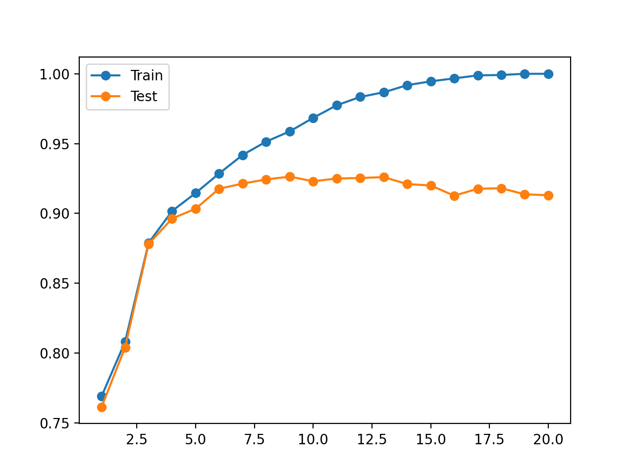
A Gentle Introduction to Machine Learning Modeling Pipelines

$
0
0

Applied machine learning is typically focused on finding a single model that performs well or best on a given dataset.

Effective use of the model will require appropriate preparation of the input data and hyperparameter tuning of the model.

Collectively, the linear sequence of steps required to prepare the data, tune the model, and transform the predictions is called the modeling pipeline. Modern machine learning libraries like the scikit-learn Python library allow this sequence of steps to be defined and used correctly (without data leakage) and consistently (during evaluation and prediction).

Nevertheless, working with modeling pipelines can be confusing to beginners as it requires a shift in perspective of the applied machine learning process.

In this tutorial, you will discover modeling pipelines for applied machine learning.

After completing this tutorial, you will know:

  • Applied machine learning is concerned with more than finding a good performing model; it also requires finding an appropriate sequence of data preparation steps and steps for the post-processing of predictions.
  • Collectively, the operations required to address a predictive modeling problem can be considered an atomic unit called a modeling pipeline.
  • Approaching applied machine learning through the lens of modeling pipelines requires a change in thinking from evaluating specific model configurations to sequences of transforms and algorithms.

Let’s get started.

A Gentle Introduction to Machine Learning Modeling Pipelines

A Gentle Introduction to Machine Learning Modeling Pipelines
Photo by Jay Huang, some rights reserved.

Tutorial Overview

This tutorial is divided into three parts; they are:

  1. Finding a Skillful Model Is Not Enough
  2. What Is a Modeling Pipeline?
  3. Implications of a Modeling Pipeline

Finding a Skillful Model Is Not Enough

Applied machine learning is the process of discovering the model that performs best for a given predictive modeling dataset.

In fact, it’s more than this.

In addition to discovering which model performs the best on your dataset, you must also discover:

  • Data transforms that best expose the unknown underlying structure of the problem to the learning algorithms.
  • Model hyperparameters that result in a good or best configuration of a chosen model.

There may also be additional considerations such as techniques that transform the predictions made by the model, like threshold moving or model calibration for predicted probabilities.

As such, it is common to think of applied machine learning as a large combinatorial search problem across data transforms, models, and model configurations.

This can be quite challenging in practice as it requires that the sequence of one or more data preparation schemes, the model, the model configuration, and any prediction transform schemes must be evaluated consistently and correctly on a given test harness.

Although tricky, it may be manageable with a simple train-test split but becomes quite unmanageable when using k-fold cross-validation or even repeated k-fold cross-validation.

The solution is to use a modeling pipeline to keep everything straight.

What Is a Modeling Pipeline?

A pipeline is a linear sequence of data preparation options, modeling operations, and prediction transform operations.

It allows the sequence of steps to be specified, evaluated, and used as an atomic unit.

  • Pipeline: A linear sequence of data preparation and modeling steps that can be treated as an atomic unit.

To make the idea clear, let’s look at two simple examples:

The first example uses data normalization for the input variables and fits a logistic regression model:

  • [Input], [Normalization], [Logistic Regression], [Predictions]

The second example standardizes the input variables, applies RFE feature selection, and fits a support vector machine.

  • [Input], [Standardization], [RFE], [SVM], [Predictions]

You can imagine other examples of modeling pipelines.

As an atomic unit, the pipeline can be evaluated using a preferred resampling scheme such as a train-test split or k-fold cross-validation.

This is important for two main reasons:

  • Avoid data leakage.
  • Consistency and reproducibility.

A modeling pipeline avoids the most common type of data leakage where data preparation techniques, such as scaling input values, are applied to the entire dataset. This is data leakage because it shares knowledge of the test dataset (such as observations that contribute to a mean or maximum known value) with the training dataset, and in turn, may result in overly optimistic model performance.

Instead, data transforms must be prepared on the training dataset only, then applied to the training dataset, test dataset, validation dataset, and any other datasets that require the transform prior to being used with the model.

A modeling pipeline ensures that the sequence of data preparation operations performed is reproducible.

Without a modeling pipeline, the data preparation steps may be performed manually twice: once for evaluating the model and once for making predictions. Any changes to the sequence must be kept consistent in both cases, otherwise differences will impact the capability and skill of the model.

A pipeline ensures that the sequence of operations is defined once and is consistent when used for model evaluation or making predictions.

The Python scikit-learn machine learning library provides a machine learning modeling pipeline via the Pipeline class.

You can learn more about how to use this Pipeline API in this tutorial:

Implications of a Modeling Pipeline

The modeling pipeline is an important tool for machine learning practitioners.

Nevertheless, there are important implications that must be considered when using them.

The main confusion for beginners when using pipelines comes in understanding what the pipeline has learned or the specific configuration discovered by the pipeline.

For example, a pipeline may use a data transform that configures itself automatically, such as the RFECV technique for feature selection.

  • When evaluating a pipeline that uses an automatically-configured data transform, what configuration does it choose? or When fitting this pipeline as a final model for making predictions, what configuration did it choose?

The answer is, it doesn’t matter.

Another example is the use of hyperparameter tuning as the final step of the pipeline.

The grid search will be performed on the data provided by any prior transform steps in the pipeline and will then search for the best combination of hyperparameters for the model using that data, then fit a model with those hyperparameters on the data.

  • When evaluating a pipeline that grid searches model hyperparameters, what configuration does it choose? or When fitting this pipeline as a final model for making predictions, what configuration did it choose?

The answer again is, it doesn’t matter.

The answer applies when using a threshold moving or probability calibration step at the end of the pipeline.

The reason is the same reason that we are not concerned about the specific internal structure or coefficients of the chosen model.

For example, when evaluating a logistic regression model, we don’t need to inspect the coefficients chosen on each k-fold cross-validation round in order to choose the model. Instead, we focus on its out-of-fold predictive skill

Similarly, when using a logistic regression model as the final model for making predictions on new data, we do not need to inspect the coefficients chosen when fitting the model on the entire dataset before making predictions.

We can inspect and discover the coefficients used by the model as an exercise in analysis, but it does not impact the selection and use of the model.

This same answer generalizes when considering a modeling pipeline.

We are not concerned about which features may have been automatically selected by a data transform in the pipeline. We are also not concerned about which hyperparameters were chosen for the model when using a grid search as the final step in the modeling pipeline.

In all three cases: the single model, the pipeline with automatic feature selection, and the pipeline with a grid search, we are evaluating the “model” or “modeling pipeline” as an atomic unit.

The pipeline allows us as machine learning practitioners to move up one level of abstraction and be less concerned with the specific outcomes of the algorithms and more concerned with the capability of a sequence of procedures.

As such, we can focus on evaluating the capability of the algorithms on the dataset, not the product of the algorithms, i.e. the model. Once we have an estimate of the pipeline, we can apply it and be confident that we will get similar performance, on average.

It is a shift in thinking and may take some time to get used to.

It is also the philosophy behind modern AutoML (automatic machine learning) techniques that treat applied machine learning as a large combinatorial search problem.

Further Reading

This section provides more resources on the topic if you are looking to go deeper.

Summary

In this tutorial, you discovered modeling pipelines for applied machine learning.

Specifically, you learned:

  • Applied machine learning is concerned with more than finding a good performing model; it also requires finding an appropriate sequence of data preparation steps and steps for the post-processing of predictions.
  • Collectively, the operations required to address a predictive modeling problem can be considered an atomic unit called a modeling pipeline.
  • Approaching applied machine learning through the lens of modeling pipelines requires a change in thinking from evaluating specific model configurations to sequences of transforms and algorithms.

Do you have any questions?
Ask your questions in the comments below and I will do my best to answer.

The post A Gentle Introduction to Machine Learning Modeling Pipelines appeared first on Machine Learning Mastery.
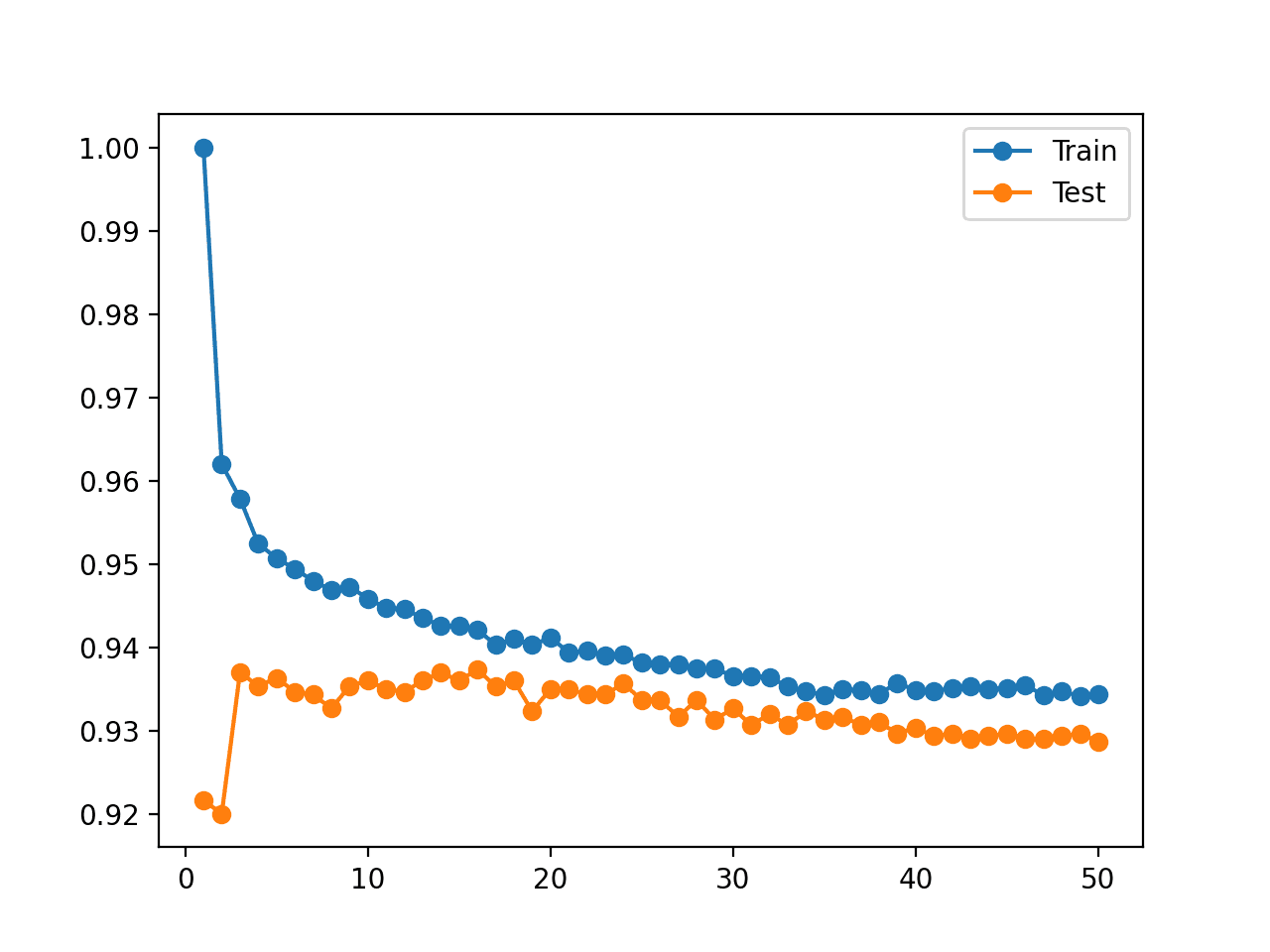

Regression Metrics for Machine Learning

$
0
0

Regression refers to predictive modeling problems that involve predicting a numeric value.

It is different from classification that involves predicting a class label. Unlike classification, you cannot use classification accuracy to evaluate the predictions made by a regression model.

Instead, you must use error metrics specifically designed for evaluating predictions made on regression problems.

In this tutorial, you will discover how to calculate error metrics for regression predictive modeling projects.

After completing this tutorial, you will know:

  • Regression predictive modeling are those problems that involve predicting a numeric value.
  • Metrics for regression involve calculating an error score to summarize the predictive skill of a model.
  • How to calculate and report mean squared error, root mean squared error, and mean absolute error.

Let’s get started.

Regression Metrics for Machine Learning

Regression Metrics for Machine Learning
Photo by Gael Varoquaux, some rights reserved.

Tutorial Overview

This tutorial is divided into three parts; they are:

  1. Regression Predictive Modeling
  2. Evaluating Regression Models
  3. Metrics for Regression
    1. Mean Squared Error
    2. Root Mean Squared Error
    3. Mean Absolute Error

Regression Predictive Modeling

Predictive modeling is the problem of developing a model using historical data to make a prediction on new data where we do not have the answer.

Predictive modeling can be described as the mathematical problem of approximating a mapping function (f) from input variables (X) to output variables (y). This is called the problem of function approximation.

The job of the modeling algorithm is to find the best mapping function we can given the time and resources available.

For more on approximating functions in applied machine learning, see the post:

Regression predictive modeling is the task of approximating a mapping function (f) from input variables (X) to a continuous output variable (y).

Regression is different from classification, which involves predicting a category or class label.

For more on the difference between classification and regression, see the tutorial:

A continuous output variable is a real-value, such as an integer or floating point value. These are often quantities, such as amounts and sizes.

For example, a house may be predicted to sell for a specific dollar value, perhaps in the range of $100,000 to $200,000.

  • A regression problem requires the prediction of a quantity.
  • A regression can have real-valued or discrete input variables.
  • A problem with multiple input variables is often called a multivariate regression problem.
  • A regression problem where input variables are ordered by time is called a time series forecasting problem.

Now that we are familiar with regression predictive modeling, let’s look at how we might evaluate a regression model.

Evaluating Regression Models

A common question by beginners to regression predictive modeling projects is:

How do I calculate accuracy for my regression model?

Accuracy (e.g. classification accuracy) is a measure for classification, not regression.

We cannot calculate accuracy for a regression model.

The skill or performance of a regression model must be reported as an error in those predictions.

This makes sense if you think about it. If you are predicting a numeric value like a height or a dollar amount, you don’t want to know if the model predicted the value exactly (this might be intractably difficult in practice); instead, we want to know how close the predictions were to the expected values.

Error addresses exactly this and summarizes on average how close predictions were to their expected values.

There are three error metrics that are commonly used for evaluating and reporting the performance of a regression model; they are:

  • Mean Squared Error (MSE).
  • Root Mean Squared Error (RMSE).
  • Mean Absolute Error (MAE)

There are many other metrics for regression, although these are the most commonly used. You can see the full list of regression metrics supported by the scikit-learn Python machine learning library here:

In the next section, let’s take a closer look at each in turn.

Metrics for Regression

In this section, we will take a closer look at the popular metrics for regression models and how to calculate them for your predictive modeling project.

Mean Squared Error

Mean Squared Error, or MSE for short, is a popular error metric for regression problems.

It is also an important loss function for algorithms fit or optimized using the least squares framing of a regression problem. Here “least squares” refers to minimizing the mean squared error between predictions and expected values.

The MSE is calculated as the mean or average of the squared differences between predicted and expected target values in a dataset.

  • MSE = 1 / N * sum for i to N (y_i – yhat_i)^2

Where y_i is the i’th expected value in the dataset and yhat_i is the i’th predicted value. The difference between these two values is squared, which has the effect of removing the sign, resulting in a positive error value.

The squaring also has the effect of inflating or magnifying large errors. That is, the larger the difference between the predicted and expected values, the larger the resulting squared positive error. This has the effect of “punishing” models more for larger errors when MSE is used as a loss function. It also has the effect of “punishing” models by inflating the average error score when used as a metric.

We can create a plot to get a feeling for how the change in prediction error impacts the squared error.

The example below gives a small contrived dataset of all 1.0 values and predictions that range from perfect (1.0) to wrong (0.0) by 0.1 increments. The squared error between each prediction and expected value is calculated and plotted to show the quadratic increase in squared error.

...
# calculate error
err = (expected[i] - predicted[i])**2

The complete example is listed below.

# example of increase in mean squared error
from matplotlib import pyplot
from sklearn.metrics import mean_squared_error
# real value
expected = [1.0, 1.0, 1.0, 1.0, 1.0, 1.0, 1.0, 1.0, 1.0, 1.0, 1.0]
# predicted value
predicted = [1.0, 0.9, 0.8, 0.7, 0.6, 0.5, 0.4, 0.3, 0.2, 0.1, 0.0]
# calculate errors
errors = list()
for i in range(len(expected)):
	# calculate error
	err = (expected[i] - predicted[i])**2
	# store error
	errors.append(err)
	# report error
	print('>%.1f, %.1f = %.3f' % (expected[i], predicted[i], err))
# plot errors
pyplot.plot(errors)
pyplot.xticks(ticks=[i for i in range(len(errors))], labels=predicted)
pyplot.xlabel('Predicted Value')
pyplot.ylabel('Mean Squared Error')
pyplot.show()

Running the example first reports the expected value, predicted value, and squared error for each case.

We can see that the error rises quickly, faster than linear (a straight line).

>1.0, 1.0 = 0.000
>1.0, 0.9 = 0.010
>1.0, 0.8 = 0.040
>1.0, 0.7 = 0.090
>1.0, 0.6 = 0.160
>1.0, 0.5 = 0.250
>1.0, 0.4 = 0.360
>1.0, 0.3 = 0.490
>1.0, 0.2 = 0.640
>1.0, 0.1 = 0.810
>1.0, 0.0 = 1.000

A line plot is created showing the curved or super-linear increase in the squared error value as the difference between the expected and predicted value is increased.

The curve is not a straight line as we might naively assume for an error metric.

Line Plot of the Increase Square Error With Predictions

Line Plot of the Increase Square Error With Predictions

The individual error terms are averaged so that we can report the performance of a model with regard to how much error the model makes generally when making predictions, rather than specifically for a given example.

The units of the MSE are squared units.

For example, if your target value represents “dollars,” then the MSE will be “squared dollars.” This can be confusing for stakeholders; therefore, when reporting results, often the root mean squared error is used instead (discussed in the next section).

The mean squared error between your expected and predicted values can be calculated using the mean_squared_error() function from the scikit-learn library.

The function takes a one-dimensional array or list of expected values and predicted values and returns the mean squared error value.

...
# calculate errors
errors = mean_squared_error(expected, predicted)

The example below gives an example of calculating the mean squared error between a list of contrived expected and predicted values.

# example of calculate the mean squared error
from sklearn.metrics import mean_squared_error
# real value
expected = [1.0, 1.0, 1.0, 1.0, 1.0, 1.0, 1.0, 1.0, 1.0, 1.0, 1.0]
# predicted value
predicted = [1.0, 0.9, 0.8, 0.7, 0.6, 0.5, 0.4, 0.3, 0.2, 0.1, 0.0]
# calculate errors
errors = mean_squared_error(expected, predicted)
# report error
print(errors)

Running the example calculates and prints the mean squared error.

0.35000000000000003

A perfect mean squared error value is 0.0, which means that all predictions matched the expected values exactly.

This is almost never the case, and if it happens, it suggests your predictive modeling problem is trivial.

A good MSE is relative to your specific dataset.

It is a good idea to first establish a baseline MSE for your dataset using a naive predictive model, such as predicting the mean target value from the training dataset. A model that achieves an MSE better than the MSE for the naive model has skill.

Root Mean Squared Error

The Root Mean Squared Error, or RMSE, is an extension of the mean squared error.

Importantly, the square root of the error is calculated, which means that the units of the RMSE are the same as the original units of the target value that is being predicted.

For example, if your target variable has the units “dollars,” then the RMSE error score will also have the unit “dollars” and not “squared dollars” like the MSE.

As such, it may be common to use MSE loss to train a regression predictive model, and to use RMSE to evaluate and report its performance.

The RMSE can be calculated as follows:

  • RMSE = sqrt(1 / N * sum for i to N (y_i – yhat_i)^2)

Where y_i is the i’th expected value in the dataset, yhat_i is the i’th predicted value, and sqrt() is the square root function.

We can restate the RMSE in terms of the MSE as:

  • RMSE = sqrt(MSE)

Note that the RMSE cannot be calculated as the average of the square root of the mean squared error values. This is a common error made by beginners and is an example of Jensen’s inequality.

You may recall that the square root is the inverse of the square operation. MSE uses the square operation to remove the sign of each error value and to punish large errors. The square root reverses this operation, although it ensures that the result remains positive.

The root mean squared error between your expected and predicted values can be calculated using the mean_squared_error() function from the scikit-learn library.

By default, the function calculates the MSE, but we can configure it to calculate the square root of the MSE by setting the “squared” argument to False.

The function takes a one-dimensional array or list of expected values and predicted values and returns the mean squared error value.

...
# calculate errors
errors = mean_squared_error(expected, predicted, squared=False)

The example below gives an example of calculating the root mean squared error between a list of contrived expected and predicted values.

# example of calculate the root mean squared error
from sklearn.metrics import mean_squared_error
# real value
expected = [1.0, 1.0, 1.0, 1.0, 1.0, 1.0, 1.0, 1.0, 1.0, 1.0, 1.0]
# predicted value
predicted = [1.0, 0.9, 0.8, 0.7, 0.6, 0.5, 0.4, 0.3, 0.2, 0.1, 0.0]
# calculate errors
errors = mean_squared_error(expected, predicted, squared=False)
# report error
print(errors)

Running the example calculates and prints the root mean squared error.

0.5916079783099616

A perfect RMSE value is 0.0, which means that all predictions matched the expected values exactly.

This is almost never the case, and if it happens, it suggests your predictive modeling problem is trivial.

A good RMSE is relative to your specific dataset.

It is a good idea to first establish a baseline RMSE for your dataset using a naive predictive model, such as predicting the mean target value from the training dataset. A model that achieves an RMSE better than the RMSE for the naive model has skill.

Mean Absolute Error

Mean Absolute Error, or MAE, is a popular metric because, like RMSE, the units of the error score match the units of the target value that is being predicted.

Unlike the RMSE, the changes in RMSE are linear and therefore intuitive.

That is, MSE and RMSE punish larger errors more than smaller errors, inflating or magnifying the mean error score. This is due to the square of the error value. The MAE does not give more or less weight to different types of errors and instead the scores increase linearly with increases in error.

As its name suggests, the MAE score is calculated as the average of the absolute error values. Absolute or abs() is a mathematical function that simply makes a number positive. Therefore, the difference between an expected and predicted value may be positive or negative and is forced to be positive when calculating the MAE.

The MAE can be calculated as follows:

  • MAE = 1 / N * sum for i to N abs(y_i – yhat_i)

Where y_i is the i’th expected value in the dataset, yhat_i is the i’th predicted value and abs() is the absolute function.

We can create a plot to get a feeling for how the change in prediction error impacts the MAE.

The example below gives a small contrived dataset of all 1.0 values and predictions that range from perfect (1.0) to wrong (0.0) by 0.1 increments. The absolute error between each prediction and expected value is calculated and plotted to show the linear increase in error.

...
# calculate error
err = abs((expected[i] - predicted[i]))

The complete example is listed below.

# plot of the increase of mean absolute error with prediction error
from matplotlib import pyplot
from sklearn.metrics import mean_squared_error
# real value
expected = [1.0, 1.0, 1.0, 1.0, 1.0, 1.0, 1.0, 1.0, 1.0, 1.0, 1.0]
# predicted value
predicted = [1.0, 0.9, 0.8, 0.7, 0.6, 0.5, 0.4, 0.3, 0.2, 0.1, 0.0]
# calculate errors
errors = list()
for i in range(len(expected)):
	# calculate error
	err = abs((expected[i] - predicted[i]))
	# store error
	errors.append(err)
	# report error
	print('>%.1f, %.1f = %.3f' % (expected[i], predicted[i], err))
# plot errors
pyplot.plot(errors)
pyplot.xticks(ticks=[i for i in range(len(errors))], labels=predicted)
pyplot.xlabel('Predicted Value')
pyplot.ylabel('Mean Absolute Error')
pyplot.show()

Running the example first reports the expected value, predicted value, and absolute error for each case.

We can see that the error rises linearly, which is intuitive and easy to understand.

>1.0, 1.0 = 0.000
>1.0, 0.9 = 0.100
>1.0, 0.8 = 0.200
>1.0, 0.7 = 0.300
>1.0, 0.6 = 0.400
>1.0, 0.5 = 0.500
>1.0, 0.4 = 0.600
>1.0, 0.3 = 0.700
>1.0, 0.2 = 0.800
>1.0, 0.1 = 0.900
>1.0, 0.0 = 1.000

A line plot is created showing the straight line or linear increase in the absolute error value as the difference between the expected and predicted value is increased.

Line Plot of the Increase Absolute Error With Predictions

Line Plot of the Increase Absolute Error With Predictions

The mean absolute error between your expected and predicted values can be calculated using the mean_absolute_error() function from the scikit-learn library.

The function takes a one-dimensional array or list of expected values and predicted values and returns the mean absolute error value.

...
# calculate errors
errors = mean_absolute_error(expected, predicted)

The example below gives an example of calculating the mean absolute error between a list of contrived expected and predicted values.

# example of calculate the mean absolute error
from sklearn.metrics import mean_absolute_error
# real value
expected = [1.0, 1.0, 1.0, 1.0, 1.0, 1.0, 1.0, 1.0, 1.0, 1.0, 1.0]
# predicted value
predicted = [1.0, 0.9, 0.8, 0.7, 0.6, 0.5, 0.4, 0.3, 0.2, 0.1, 0.0]
# calculate errors
errors = mean_absolute_error(expected, predicted)
# report error
print(errors)

Running the example calculates and prints the mean absolute error.

0.5

A perfect mean absolute error value is 0.0, which means that all predictions matched the expected values exactly.

This is almost never the case, and if it happens, it suggests your predictive modeling problem is trivial.

A good MAE is relative to your specific dataset.

It is a good idea to first establish a baseline MAE for your dataset using a naive predictive model, such as predicting the mean target value from the training dataset. A model that achieves a MAE better than the MAE for the naive model has skill.

Further Reading

This section provides more resources on the topic if you are looking to go deeper.

Tutorials

APIs

Articles

Summary

In this tutorial, you discovered how to calculate error for regression predictive modeling projects.

Specifically, you learned:

  • Regression predictive modeling are those problems that involve predicting a numeric value.
  • Metrics for regression involve calculating an error score to summarize the predictive skill of a model.
  • How to calculate and report mean squared error, root mean squared error, and mean absolute error.

Do you have any questions?
Ask your questions in the comments below and I will do my best to answer.

The post Regression Metrics for Machine Learning appeared first on Machine Learning Mastery.

Sensitivity Analysis of Dataset Size vs. Model Performance

$
0
0

Machine learning model performance often improves with dataset size for predictive modeling.

This depends on the specific datasets and on the choice of model, although it often means that using more data can result in better performance and that discoveries made using smaller datasets to estimate model performance often scale to using larger datasets.

The problem is the relationship is unknown for a given dataset and model, and may not exist for some datasets and models. Additionally, if such a relationship does exist, there may be a point or points of diminishing returns where adding more data may not improve model performance or where datasets are too small to effectively capture the capability of a model at a larger scale.

These issues can be addressed by performing a sensitivity analysis to quantify the relationship between dataset size and model performance. Once calculated, we can interpret the results of the analysis and make decisions about how much data is enough, and how small a dataset may be to effectively estimate performance on larger datasets.

In this tutorial, you will discover how to perform a sensitivity analysis of dataset size vs. model performance.

After completing this tutorial, you will know:

  • Selecting a dataset size for machine learning is a challenging open problem.
  • Sensitivity analysis provides an approach to quantifying the relationship between model performance and dataset size for a given model and prediction problem.
  • How to perform a sensitivity analysis of dataset size and interpret the results.

Let’s get started.

Sensitivity Analysis of Dataset Size vs. Model Performance

Sensitivity Analysis of Dataset Size vs. Model Performance
Photo by Graeme Churchard, some rights reserved.

Tutorial Overview

This tutorial is divided into three parts; they are:

  1. Dataset Size Sensitivity Analysis
  2. Synthetic Prediction Task and Baseline Model
  3. Sensitivity Analysis of Dataset Size

Dataset Size Sensitivity Analysis

The amount of training data required for a machine learning predictive model is an open question.

It depends on your choice of model, on the way you prepare the data, and on the specifics of the data itself.

For more on the challenge of selecting a training dataset size, see the tutorial:

One way to approach this problem is to perform a sensitivity analysis and discover how the performance of your model on your dataset varies with more or less data.

This might involve evaluating the same model with different sized datasets and looking for a relationship between dataset size and performance or a point of diminishing returns.

Typically, there is a strong relationship between training dataset size and model performance, especially for nonlinear models. The relationship often involves an improvement in performance to a point and a general reduction in the expected variance of the model as the dataset size is increased.

Knowing this relationship for your model and dataset can be helpful for a number of reasons, such as:

  • Evaluate more models.
  • Find a better model.
  • Decide to gather more data.

You can evaluate a large number of models and model configurations quickly on a smaller sample of the dataset with confidence that the performance will likely generalize in a specific way to a larger training dataset.

This may allow evaluating many more models and configurations than you may otherwise be able to given the time available, and in turn, perhaps discover a better overall performing model.

You may also be able to generalize and estimate the expected performance of model performance to much larger datasets and estimate whether it is worth the effort or expense of gathering more training data.

Now that we are familiar with the idea of performing a sensitivity analysis of model performance to dataset size, let’s look at a worked example.

Synthetic Prediction Task and Baseline Model

Before we dive into a sensitivity analysis, let’s select a dataset and baseline model for the investigation.

We will use a synthetic binary (two-class) classification dataset in this tutorial. This is ideal as it allows us to scale the number of generated samples for the same problem as needed.

The make_classification() scikit-learn function can be used to create a synthetic classification dataset. In this case, we will use 20 input features (columns) and generate 1,000 samples (rows). The seed for the pseudo-random number generator is fixed to ensure the same base “problem” is used each time samples are generated.

The example below generates the synthetic classification dataset and summarizes the shape of the generated data.

# test classification dataset
from sklearn.datasets import make_classification
# define dataset
X, y = make_classification(n_samples=1000, n_features=20, n_informative=15, n_redundant=5, random_state=1)
# summarize the dataset
print(X.shape, y.shape)

Running the example generates the data and reports the size of the input and output components, confirming the expected shape.

(1000, 20) (1000,)

Next, we can evaluate a predictive model on this dataset.

We will use a decision tree (DecisionTreeClassifier) as the predictive model. It was chosen because it is a nonlinear algorithm and has a high variance, which means that we would expect performance to improve with increases in the size of the training dataset.

We will use a best practice of repeated stratified k-fold cross-validation to evaluate the model on the dataset, with 3 repeats and 10 folds.

The complete example of evaluating the decision tree model on the synthetic classification dataset is listed below.

# evaluate a decision tree model on the synthetic classification dataset
from sklearn.datasets import make_classification
from sklearn.model_selection import cross_val_score
from sklearn.model_selection import RepeatedStratifiedKFold
from sklearn.tree import DecisionTreeClassifier
# load dataset
X, y = make_classification(n_samples=1000, n_features=20, n_informative=15, n_redundant=5, random_state=1)
# define model evaluation procedure
cv = RepeatedStratifiedKFold(n_splits=10, n_repeats=3, random_state=1)
# define model
model = DecisionTreeClassifier()
# evaluate model
scores = cross_val_score(model, X, y, scoring='accuracy', cv=cv, n_jobs=-1)
# report performance
print('Mean Accuracy: %.3f (%.3f)' % (scores.mean(), scores.std()))

Running the example creates the dataset then estimates the performance of the model on the problem using the chosen test harness.

Note: Your results may vary given the stochastic nature of the algorithm or evaluation procedure, or differences in numerical precision. Consider running the example a few times and compare the average outcome.

In this case, we can see that the mean classification accuracy is about 82.7%.

Mean Accuracy: 0.827 (0.042)

Next, let’s look at how we might perform a sensitivity analysis of dataset size on model performance.

Sensitivity Analysis of Dataset Size

The previous section showed how to evaluate a chosen model on the available dataset.

It raises questions, such as:

Will the model perform better on more data?

More generally, we may have sophisticated questions such as:

Does the estimated performance hold on smaller or larger samples from the problem domain?

These are hard questions to answer, but we can approach them by using a sensitivity analysis. Specifically, we can use a sensitivity analysis to learn:

How sensitive is model performance to dataset size?

Or more generally:

What is the relationship of dataset size to model performance?

There are many ways to perform a sensitivity analysis, but perhaps the simplest approach is to define a test harness to evaluate model performance and then evaluate the same model on the same problem with differently sized datasets.

This will allow the train and test portions of the dataset to increase with the size of the overall dataset.

To make the code easier to read, we will split it up into functions.

First, we can define a function that will prepare (or load) the dataset of a given size. The number of rows in the dataset is specified by an argument to the function.

If you are using this code as a template, this function can be changed to load your dataset from file and select a random sample of a given size.

# load dataset
def load_dataset(n_samples):
	# define the dataset
	X, y = make_classification(n_samples=int(n_samples), n_features=20, n_informative=15, n_redundant=5, random_state=1)
	return X, y

Next, we need a function to evaluate a model on a loaded dataset.

We will define a function that takes a dataset and returns a summary of the performance of the model evaluated using the test harness on the dataset.

This function is listed below, taking the input and output elements of a dataset and returning the mean and standard deviation of the decision tree model on the dataset.

# evaluate a model
def evaluate_model(X, y):
	# define model evaluation procedure
	cv = RepeatedStratifiedKFold(n_splits=10, n_repeats=3, random_state=1)
	# define model
	model = DecisionTreeClassifier()
	# evaluate model
	scores = cross_val_score(model, X, y, scoring='accuracy', cv=cv, n_jobs=-1)
	# return summary stats
	return [scores.mean(), scores.std()]

Next, we can define a range of different dataset sizes to evaluate.

The sizes should be chosen proportional to the amount of data you have available and the amount of running time you are willing to expend.

In this case, we will keep the sizes modest to limit running time, from 50 to one million rows on a rough log10 scale.

...
# define number of samples to consider
sizes = [50, 100, 500, 1000, 5000, 10000, 50000, 100000, 500000, 1000000]

Next, we can enumerate each dataset size, create the dataset, evaluate a model on the dataset, and store the results for later analysis.

...
# evaluate each number of samples
means, stds = list(), list()
for n_samples in sizes:
	# get a dataset
	X, y = load_dataset(n_samples)
	# evaluate a model on this dataset size
	mean, std = evaluate_model(X, y)
	# store
	means.append(mean)
	stds.append(std)

Next, we can summarize the relationship between the dataset size and model performance.

In this case, we will simply plot the result with error bars so we can spot any trends visually.

We will use the standard deviation as a measure of uncertainty on the estimated model performance. This can be achieved by multiplying the value by 2 to cover approximately 95% of the expected performance if the performance follows a normal distribution.

This can be shown on the plot as an error bar around the mean expected performance for a dataset size.

...
# define error bar as 2 standard deviations from the mean or 95%
err = [min(1, s * 2) for s in stds]
# plot dataset size vs mean performance with error bars
pyplot.errorbar(sizes, means, yerr=err, fmt='-o')

To make the plot more readable, we can change the scale of the x-axis to log, given that our dataset sizes are on a rough log10 scale.

...
# change the scale of the x-axis to log
ax = pyplot.gca()
ax.set_xscale("log", nonpositive='clip')
# show the plot
pyplot.show()

And that’s it.

We would generally expect mean model performance to increase with dataset size. We would also expect the uncertainty in model performance to decrease with dataset size.

Tying this all together, the complete example of performing a sensitivity analysis of dataset size on model performance is listed below.

# sensitivity analysis of model performance to dataset size
from sklearn.datasets import make_classification
from sklearn.model_selection import cross_val_score
from sklearn.model_selection import RepeatedStratifiedKFold
from sklearn.tree import DecisionTreeClassifier
from matplotlib import pyplot

# load dataset
def load_dataset(n_samples):
	# define the dataset
	X, y = make_classification(n_samples=int(n_samples), n_features=20, n_informative=15, n_redundant=5, random_state=1)
	return X, y

# evaluate a model
def evaluate_model(X, y):
	# define model evaluation procedure
	cv = RepeatedStratifiedKFold(n_splits=10, n_repeats=3, random_state=1)
	# define model
	model = DecisionTreeClassifier()
	# evaluate model
	scores = cross_val_score(model, X, y, scoring='accuracy', cv=cv, n_jobs=-1)
	# return summary stats
	return [scores.mean(), scores.std()]

# define number of samples to consider
sizes = [50, 100, 500, 1000, 5000, 10000, 50000, 100000, 500000, 1000000]
# evaluate each number of samples
means, stds = list(), list()
for n_samples in sizes:
	# get a dataset
	X, y = load_dataset(n_samples)
	# evaluate a model on this dataset size
	mean, std = evaluate_model(X, y)
	# store
	means.append(mean)
	stds.append(std)
	# summarize performance
	print('>%d: %.3f (%.3f)' % (n_samples, mean, std))
# define error bar as 2 standard deviations from the mean or 95%
err = [min(1, s * 2) for s in stds]
# plot dataset size vs mean performance with error bars
pyplot.errorbar(sizes, means, yerr=err, fmt='-o')
# change the scale of the x-axis to log
ax = pyplot.gca()
ax.set_xscale("log", nonpositive='clip')
# show the plot
pyplot.show()

Running the example reports the status along the way of dataset size vs. estimated model performance.

Note: Your results may vary given the stochastic nature of the algorithm or evaluation procedure, or differences in numerical precision. Consider running the example a few times and compare the average outcome.

In this case, we can see the expected trend of increasing mean model performance with dataset size and decreasing model variance measured using the standard deviation of classification accuracy.

We can see that there is perhaps a point of diminishing returns in estimating model performance at perhaps 10,000 or 50,000 rows.

Specifically, we do see an improvement in performance with more rows, but we can probably capture this relationship with little variance with 10K or 50K rows of data.

We can also see a drop-off in estimated performance with 1,000,000 rows of data, suggesting that we are probably maxing out the capability of the model above 100,000 rows and are instead measuring statistical noise in the estimate.

This might mean an upper bound on expected performance and likely that more data beyond this point will not improve the specific model and configuration on the chosen test harness.

>50: 0.673 (0.141)
>100: 0.703 (0.135)
>500: 0.809 (0.055)
>1000: 0.826 (0.044)
>5000: 0.835 (0.016)
>10000: 0.866 (0.011)
>50000: 0.900 (0.005)
>100000: 0.912 (0.003)
>500000: 0.938 (0.001)
>1000000: 0.936 (0.001)

The plot makes the relationship between dataset size and estimated model performance much clearer.

The relationship is nearly linear with a log dataset size. The change in the uncertainty shown as the error bar also dramatically decreases on the plot from very large values with 50 or 100 samples, to modest values with 5,000 and 10,000 samples and practically gone beyond these sizes.

Given the modest spread with 5,000 and 10,000 samples and the practically log-linear relationship, we could probably get away with using 5K or 10K rows to approximate model performance.

Line Plot With Error Bars of Dataset Size vs. Model Performance

Line Plot With Error Bars of Dataset Size vs. Model Performance

We could use these findings as the basis for testing additional model configurations and even different model types.

The danger is that different models may perform very differently with more or less data and it may be wise to repeat the sensitivity analysis with a different chosen model to confirm the relationship holds. Alternately, it may be interesting to repeat the analysis with a suite of different model types.

Further Reading

This section provides more resources on the topic if you are looking to go deeper.

Tutorials

APIs

Articles

Summary

In this tutorial, you discovered how to perform a sensitivity analysis of dataset size vs. model performance.

Specifically, you learned:

  • Selecting a dataset size for machine learning is a challenging open problem.
  • Sensitivity analysis provides an approach to quantifying the relationship between model performance and dataset size for a given model and prediction problem.
  • How to perform a sensitivity analysis of dataset size and interpret the results.

Do you have any questions?
Ask your questions in the comments below and I will do my best to answer.

The post Sensitivity Analysis of Dataset Size vs. Model Performance appeared first on Machine Learning Mastery.

What Is Semi-Supervised Learning

$
0
0

Semi-supervised learning is a learning problem that involves a small number of labeled examples and a large number of unlabeled examples.

Learning problems of this type are challenging as neither supervised nor unsupervised learning algorithms are able to make effective use of the mixtures of labeled and untellable data. As such, specialized semis-supervised learning algorithms are required.

In this tutorial, you will discover a gentle introduction to the field of semi-supervised learning for machine learning.

After completing this tutorial, you will know:

  • Semi-supervised learning is a type of machine learning that sits between supervised and unsupervised learning.
  • Top books on semi-supervised learning designed to get you up to speed in the field.
  • Additional resources on semi-supervised learning, such as review papers and APIs.

Let’s get started.

What Is Semi-Supervised Learning

What Is Semi-Supervised Learning
Photo by Paul VanDerWerf, some rights reserved.

Tutorial Overview

This tutorial is divided into three parts; they are:

  1. Semi-Supervised Learning
  2. Books on Semi-Supervised Learning
  3. Additional Resources

Semi-Supervised Learning

Semi-supervised learning is a type of machine learning.

It refers to a learning problem (and algorithms designed for the learning problem) that involves a small portion of labeled examples and a large number of unlabeled examples from which a model must learn and make predictions on new examples.

… dealing with the situation where relatively few labeled training points are available, but a large number of unlabeled points are given, it is directly relevant to a multitude of practical problems where it is relatively expensive to produce labeled data …

— Page xiii, Semi-Supervised Learning, 2006.

As such, it is a learning problem that sits between supervised learning and unsupervised learning.

Semi-supervised learning (SSL) is halfway between supervised and unsupervised learning. In addition to unlabeled data, the algorithm is provided with some super- vision information – but not necessarily for all examples. Often, this information will be the targets associated with some of the examples.

— Page 2, Semi-Supervised Learning, 2006.

We require semi-supervised learning algorithms when working with data where labeling examples is challenging or expensive.

Semi-supervised learning has tremendous practical value. In many tasks, there is a paucity of labeled data. The labels y may be difficult to obtain because they require human annotators, special devices, or expensive and slow experiments.

— Page 9, Introduction to Semi-Supervised Learning, 2009.

The sign of an effective semi-supervised learning algorithm is that it can achieve better performance than a supervised learning algorithm fit only on the labeled training examples.

Semi-supervised learning algorithms generally are able to clear this low bar expectation.

… in comparison with a supervised algorithm that uses only labeled data, can one hope to have a more accurate prediction by taking into account the unlabeled points? […] in principle the answer is ‘yes.’”

— Page 4, Semi-Supervised Learning, 2006.

Finally, semi-supervised learning may be used or may contrast inductive and transductive learning.

Generally, inductive learning refers to a learning algorithm that learns from labeled training data and generalizes to new data, such as a test dataset. Transductive learning refers to learning from labeled training data and generalizing to available unlabeled (training) data. Both types of learning tasks may be performed by a semi-supervised learning algorithm.

… there are two distinct goals. One is to predict the labels on future test data. The other goal is to predict the labels on the unlabeled instances in the training sample. We call the former inductive semi-supervised learning, and the latter transductive learning.

— Page 12, Introduction to Semi-Supervised Learning, 2009.

If you are new to the idea of transduction vs. induction, the following tutorial has more information:

Now that we are familiar with semi-supervised learning from a high-level, let’s take a look at top books on the topic.

Books on Semi-Supervised Learning

Semi-supervised learning is a new and fast-moving field of study, and as such, there are very few books on the topic.

There are perhaps two key books on semi-supervised learning that you should consider if you are new to the topic; they are:

Let’s take a closer look at each in turn.

Semi-Supervised Learning, 2006

The book “Semi-Supervised Learning” was published in 2006 and was edited by Olivier Chapelle, Bernhard Scholkopf, and Alexander Zien.

Semi-Supervised Learning

Semi-Supervised Learning

This book provides a large number of chapters, each written by top researchers in the field.

It is designed to take you on a tour of the field of research including intuitions, top techniques, and open problems.

The full table of contents is listed below.

Table of Contents

  • Chapter 01: Introduction to Semi-Supervised Learning
  • Part I: Generative Models
    • Chapter 02: A Taxonomy for Semi-Supervised Learning Methods
    • Chapter 03: Semi-Supervised Text Classification Using EM
    • Chapter 04: Risks of Semi-Supervised Learning
    • Chapter 05: Probabilistic Semi-Supervised Clustering with Constraints
  • Part II: Low-Density Separation
    • Chapter 06: Transductive Support Vector Machines
    • Chapter 07: Semi-Supervised Learning Using Semi-Definite Programming
    • Chapter 08: Gaussian Processes and the Null-Category Noise Model
    • Chapter 09: Entropy Regularization
    • Chapter 10: Data-Dependent Regularization
  • Part III: Graph-Based Methods
    • Chapter 11: Label Propagation and Quadratic Criterion
    • Chapter 12: The Geometric Basis of Semi-Supervised Learning
    • Chapter 13: Discrete Regularization
    • Chapter 14: Semi-Supervised Learning with Conditional Harmonic Mixing
  • Part IV: Change of Representation
    • Chapter 15: Graph Kernels by Spectral Transforms
    • Chapter 16: Spectral Methods for Dimensionality Reduction
    • Chapter 17: Modifying Distances
  • Part V: Semi-Supervised Learning in Practice
    • Chapter 18: Large-Scale Algorithms
    • Chapter 19: Semi-Supervised Protein Classification Using Cluster Kernels
    • Chapter 20: Prediction of Protein Function from Networks
    • Chapter 21: Analysis of Benchmarks
  • Part VI: Perspectives
    • Chapter 22: An Augmented PAC Model for Semi-Supervised Learning
    • Chapter 23: Metric-Based Approaches for Semi-Supervised Regression and Classification
    • Chapter 24: Transductive Inference and Semi-Supervised Learning
    • Chapter 25: A Discussion of Semi-Supervised Learning and Transduction

I highly recommend this book and reading it cover to cover if you are starting out in this field.

Introduction to Semi-Supervised Learning, 2009

The book “Introduction to Semi-Supervised Learning” was published in 2009 and was written by Xiaojin Zhu and Andrew Goldberg.

Introduction to Semi-Supervised Learning

Introduction to Semi-Supervised Learning

This book is aimed at students, researchers, and engineers just getting started in the field.

The book is a beginner’s guide to semi-supervised learning. It is aimed at advanced under-graduates, entry-level graduate students and researchers in areas as diverse as Computer Science, Electrical Engineering, Statistics, and Psychology.

— Page xiii, Introduction to Semi-Supervised Learning, 2009.

It’s a shorter read than the above book and a great introduction.

The full table of contents is listed below.

Table of Contents

  • Chapter 01: Introduction to Statistical Machine Learning
  • Chapter 02: Overview of Semi-Supervised Learning
  • Chapter 03: Mixture Models and EM
  • Chapter 04: Co-Training
  • Chapter 05: Graph-Based Semi-Supervised Learning
  • Chapter 06: Semi-Supervised Support Vector Machines
  • Chapter 07: Human Semi-Supervised Learning
  • Chapter 08: Theory and Outlook

I also recommend this book if you’re just starting out for a quick review of the key elements of the field.

Other Books

There are some additional books on semi-supervised learning that you might also like to consider; they are:

Have you read any of the above books?
What did you think?

Did I miss your favorite book?
Let me know in the comments below.

Additional Resources

There are additional resources that may be helpful when getting started in the field of semi-supervised learning.

I would recommend reading some review papers.

Some examples of good review papers on semi-supervised learning include:

In this paper, we provide a comprehensive overview of deep semi-supervised learning, starting with an introduction to the field, followed by a summarization of the dominant semi-supervised approaches in deep learning.

An Overview of Deep Semi-Supervised Learning, 2020.

An Overview of Deep Semi-Supervised Learning

An Overview of Deep Semi-Supervised Learning

It is also a good idea to try out some of the algorithms.

The scikit-learn Python machine learning library provides a few graph-based semi-supervised learning algorithms that you can try:

The Wikipedia article may also provide some useful links for further reading:

Summary

In this tutorial, you discovered a gentle introduction to the field of semi-supervised learning for machine learning.

Specifically, you learned:

  • Semi-supervised learning is a type of machine learning that sits between supervised and unsupervised learning.
  • Top books on semi-supervised learning designed to get you up to speed in the field.
  • Additional resources on semi-supervised learning, such as review papers and APIs.

Do you have any questions?
Ask your questions in the comments below and I will do my best to answer.

The post What Is Semi-Supervised Learning appeared first on Machine Learning Mastery.

How to Develop LARS Regression Models in Python

$
0
0

Regression is a modeling task that involves predicting a numeric value given an input.

Linear regression is the standard algorithm for regression that assumes a linear relationship between inputs and the target variable. An extension to linear regression involves adding penalties to the loss function during training that encourage simpler models that have smaller coefficient values. These extensions are referred to as regularized linear regression or penalized linear regression.

Lasso Regression is a popular type of regularized linear regression that includes an L1 penalty. This has the effect of shrinking the coefficients for those input variables that do not contribute much to the prediction task.

Least Angle Regression or LARS for short provides an alternate, efficient way of fitting a Lasso regularized regression model that does not require any hyperparameters.

In this tutorial, you will discover how to develop and evaluate LARS Regression models in Python.

After completing this tutorial, you will know:

  • LARS Regression provides an alternate way to train a Lasso regularized linear regression model that adds a penalty to the loss function during training.
  • How to evaluate a LARS Regression model and use a final model to make predictions for new data.
  • How to configure the LARS Regression model for a new dataset automatically using a cross-validation version of the estimator.

Let’s get started.

How to Develop LARS Regression Models in Python

How to Develop LARS Regression Models in Python
Photo by Nicolas Raymond, some rights reserved.

Tutorial Overview

This tutorial is divided into three parts; they are:

  1. LARS Regression
  2. Example of LARS Regression
  3. Tuning LARS Hyperparameters

LARS Regression

Linear regression refers to a model that assumes a linear relationship between input variables and the target variable.

With a single input variable, this relationship is a line, and with higher dimensions, this relationship can be thought of as a hyperplane that connects the input variables to the target variable. The coefficients of the model are found via an optimization process that seeks to minimize the sum squared error between the predictions (yhat) and the expected target values (y).

  • loss = sum i=0 to n (y_i – yhat_i)^2

A problem with linear regression is that estimated coefficients of the model can become large, making the model sensitive to inputs and possibly unstable. This is particularly true for problems with few observations (samples) or more input predictors (p) than variables than samples (n)  (so-called p >> n problems).

One approach to address the stability of regression models is to change the loss function to include additional costs for a model that has large coefficients. Linear regression models that use these modified loss functions during training are referred to collectively as penalized linear regression.

A popular penalty is to penalize a model based on the sum of the absolute coefficient values. This is called the L1 penalty. An L1 penalty minimizes the size of all coefficients and allows some coefficients to be minimized to the value zero, which removes the predictor from the model.

  • l1_penalty = sum j=0 to p abs(beta_j)

An L1 penalty minimizes the size of all coefficients and allows any coefficient to go to the value of zero, effectively removing input features from the model. This acts as a type of automatic feature selection method.

… a consequence of penalizing the absolute values is that some parameters are actually set to 0 for some value of lambda. Thus the lasso yields models that simultaneously use regularization to improve the model and to conduct feature selection.

— Page 125, Applied Predictive Modeling, 2013.

This penalty can be added to the cost function for linear regression and is referred to as Least Absolute Shrinkage And Selection Operator (LASSO), or more commonly, “Lasso” (with title case) for short.

The Lasso trains the model using a least-squares loss training procedure.

Least Angle Regression, LAR or LARS for short, is an alternative approach to solving the optimization problem of fitting the penalized model. Technically, LARS is a forward stepwise version of feature selection for regression that can be adapted for the Lasso model.

Unlike the Lasso, it does not require a hyperparameter that controls the weighting of the penalty in the loss function. Instead, the weighting is discovered automatically by LARS.

… least angle regression (LARS), is a broad framework that encompasses the lasso and similar models. The LARS model can be used to fit lasso models more efficiently, especially in high-dimensional problems.

— Page 126, Applied Predictive Modeling, 2013.

Now that we are familiar with LARS penalized regression, let’s look at a worked example.

Example of LARS Regression

In this section, we will demonstrate how to use the LARS Regression algorithm.

First, let’s introduce a standard regression dataset. We will use the housing dataset.

The housing dataset is a standard machine learning dataset comprising 506 rows of data with 13 numerical input variables and a numerical target variable.

Using a test harness of repeated stratified 10-fold cross-validation with three repeats, a naive model can achieve a mean absolute error (MAE) of about 6.6. A top-performing model can achieve a MAE on this same test harness of about 1.9. This provides the bounds of expected performance on this dataset.

The dataset involves predicting the house price given details of the house’s suburb in the American city of Boston.

No need to download the dataset; we will download it automatically as part of our worked examples.

The example below downloads and loads the dataset as a Pandas DataFrame and summarizes the shape of the dataset and the first five rows of data.

# load and summarize the housing dataset
from pandas import read_csv
from matplotlib import pyplot
# load dataset
url = 'https://raw.githubusercontent.com/jbrownlee/Datasets/master/housing.csv'
dataframe = read_csv(url, header=None)
# summarize shape
print(dataframe.shape)
# summarize first few lines
print(dataframe.head())

Running the example confirms the 506 rows of data and 13 input variables and a single numeric target variable (14 in total). We can also see that all input variables are numeric.

(506, 14)
        0     1     2   3      4      5   ...  8      9     10      11    12    13
0  0.00632  18.0  2.31   0  0.538  6.575  ...   1  296.0  15.3  396.90  4.98  24.0
1  0.02731   0.0  7.07   0  0.469  6.421  ...   2  242.0  17.8  396.90  9.14  21.6
2  0.02729   0.0  7.07   0  0.469  7.185  ...   2  242.0  17.8  392.83  4.03  34.7
3  0.03237   0.0  2.18   0  0.458  6.998  ...   3  222.0  18.7  394.63  2.94  33.4
4  0.06905   0.0  2.18   0  0.458  7.147  ...   3  222.0  18.7  396.90  5.33  36.2

[5 rows x 14 columns]

The scikit-learn Python machine learning library provides an implementation of the LARS penalized regression algorithm via the Lars class.

...
# define model
model = Lars()

We can evaluate the LARS Regression model on the housing dataset using repeated 10-fold cross-validation and report the average mean absolute error (MAE) on the dataset.

# evaluate an lars regression model on the dataset
from numpy import mean
from numpy import std
from numpy import absolute
from pandas import read_csv
from sklearn.model_selection import cross_val_score
from sklearn.model_selection import RepeatedKFold
from sklearn.linear_model import Lars
# load the dataset
url = 'https://raw.githubusercontent.com/jbrownlee/Datasets/master/housing.csv'
dataframe = read_csv(url, header=None)
data = dataframe.values
X, y = data[:, :-1], data[:, -1]
# define model
model = Lars()
# define model evaluation method
cv = RepeatedKFold(n_splits=10, n_repeats=3, random_state=1)
# evaluate model
scores = cross_val_score(model, X, y, scoring='neg_mean_absolute_error', cv=cv, n_jobs=-1)
# force scores to be positive
scores = absolute(scores)
print('Mean MAE: %.3f (%.3f)' % (mean(scores), std(scores)))

Running the example evaluates the LARS Regression algorithm on the housing dataset and reports the average MAE across the three repeats of 10-fold cross-validation.

Your specific results may vary given the stochastic nature of the learning algorithm. Consider running the example a few times.

In this case, we can see that the model achieved a MAE of about 3.432.

Mean MAE: 3.432 (0.552)

We may decide to use the LARS Regression as our final model and make predictions on new data.

This can be achieved by fitting the model on all available data and calling the predict() function, passing in a new row of data.

We can demonstrate this with a complete example, listed below.

# make a prediction with a lars regression model on the dataset
from pandas import read_csv
from sklearn.linear_model import Lars
# load the dataset
url = 'https://raw.githubusercontent.com/jbrownlee/Datasets/master/housing.csv'
dataframe = read_csv(url, header=None)
data = dataframe.values
X, y = data[:, :-1], data[:, -1]
# define model
model = Lars()
# fit model
model.fit(X, y)
# define new data
row = [0.00632,18.00,2.310,0,0.5380,6.5750,65.20,4.0900,1,296.0,15.30,396.90,4.98]
# make a prediction
yhat = model.predict([row])
# summarize prediction
print('Predicted: %.3f' % yhat)

Running the example fits the model and makes a prediction for the new rows of data.

Your specific results may vary given the stochastic nature of the learning algorithm. Try running the example a few times.

Predicted: 29.904

Next, we can look at configuring the model hyperparameters.

Tuning LARS Hyperparameters

As part of the LARS training algorithm, it automatically discovers the best value for the lambda hyperparameter used in the Lasso algorithm.

This hyperparameter is referred to as the “alpha” argument in the scikit-learn implementation of Lasso and LARS.

Nevertheless, the process of automatically discovering the best model and alpha hyperparameter is still based on a single training dataset.

An alternative approach is to fit the model on multiple subsets of the training dataset and choose the best internal model configuration across the folds, in this case, the value of alpha. Generally, this is referred to as a cross-validation estimator.

The scikit-learn libraries offer a cross-validation version of the LARS for finding a more robust value for alpha via the LarsCV class.

The example below demonstrates how to fit a LarsCV model and report the alpha value found via cross-validation

# use automatically configured the lars regression algorithm
from numpy import arange
from pandas import read_csv
from sklearn.linear_model import LarsCV
from sklearn.model_selection import RepeatedKFold
# load the dataset
url = 'https://raw.githubusercontent.com/jbrownlee/Datasets/master/housing.csv'
dataframe = read_csv(url, header=None)
data = dataframe.values
X, y = data[:, :-1], data[:, -1]
# define model evaluation method
cv = RepeatedKFold(n_splits=10, n_repeats=3, random_state=1)
# define model
model = LarsCV(cv=cv, n_jobs=-1)
# fit model
model.fit(X, y)
# summarize chosen configuration
print('alpha: %f' % model.alpha_)

Running the example fits the LarsCV model using repeated cross-validation and reports an optimal alpha value found across the runs.

alpha: 0.001623

This version of the LARS model may prove more robust in practice.

We can evaluate it using the same procedure we did in the previous section, although in this case, each model fit is based on the hyperparameters found via repeated k-fold cross-validation internally (e.g. cross-validation of a cross-validation estimator).

The complete example is listed below.

# evaluate an lars cross-validation regression model on the dataset
from numpy import mean
from numpy import std
from numpy import absolute
from pandas import read_csv
from sklearn.model_selection import cross_val_score
from sklearn.model_selection import RepeatedKFold
from sklearn.linear_model import LarsCV
# load the dataset
url = 'https://raw.githubusercontent.com/jbrownlee/Datasets/master/housing.csv'
dataframe = read_csv(url, header=None)
data = dataframe.values
X, y = data[:, :-1], data[:, -1]
# define model evaluation method
cv = RepeatedKFold(n_splits=10, n_repeats=3, random_state=1)
# define model
model = LarsCV(cv=cv, n_jobs=-1)
# evaluate model
scores = cross_val_score(model, X, y, scoring='neg_mean_absolute_error', cv=cv, n_jobs=-1)
# force scores to be positive
scores = absolute(scores)
print('Mean MAE: %.3f (%.3f)' % (mean(scores), std(scores)))

Running the example will evaluate the cross-validated estimation of model hyperparameters using repeated cross-validation.

Your specific results may vary given the stochastic nature of the learning algorithm. Try running the example a few times.

In this case, we can see that we achieved slightly better results with 3.374 vs. 3.432 in the previous section.

Mean MAE: 3.374 (0.558)

Further Reading

This section provides more resources on the topic if you are looking to go deeper.

Books

APIs

Articles

Summary

In this tutorial, you discovered how to develop and evaluate LARS Regression models in Python.

Specifically, you learned:

  • LARS Regression provides an alternate way to train a Lasso regularized linear regression model that adds a penalty to the loss function during training.
  • How to evaluate a LARS Regression model and use a final model to make predictions for new data.
  • How to configure the LARS Regression model for a new dataset automatically using a cross-validation version of the estimator.

Do you have any questions?
Ask your questions in the comments below and I will do my best to answer.

The post How to Develop LARS Regression Models in Python appeared first on Machine Learning Mastery.

What Is Semi-Supervised Learning

$
0
0

Semi-supervised learning is a learning problem that involves a small number of labeled examples and a large number of unlabeled examples.

Learning problems of this type are challenging as neither supervised nor unsupervised learning algorithms are able to make effective use of the mixtures of labeled and untellable data. As such, specialized semis-supervised learning algorithms are required.

In this tutorial, you will discover a gentle introduction to the field of semi-supervised learning for machine learning.

After completing this tutorial, you will know:

  • Semi-supervised learning is a type of machine learning that sits between supervised and unsupervised learning.
  • Top books on semi-supervised learning designed to get you up to speed in the field.
  • Additional resources on semi-supervised learning, such as review papers and APIs.

Let’s get started.

What Is Semi-Supervised Learning

What Is Semi-Supervised Learning
Photo by Paul VanDerWerf, some rights reserved.

Tutorial Overview

This tutorial is divided into three parts; they are:

  1. Semi-Supervised Learning
  2. Books on Semi-Supervised Learning
  3. Additional Resources

Semi-Supervised Learning

Semi-supervised learning is a type of machine learning.

It refers to a learning problem (and algorithms designed for the learning problem) that involves a small portion of labeled examples and a large number of unlabeled examples from which a model must learn and make predictions on new examples.

… dealing with the situation where relatively few labeled training points are available, but a large number of unlabeled points are given, it is directly relevant to a multitude of practical problems where it is relatively expensive to produce labeled data …

— Page xiii, Semi-Supervised Learning, 2006.

As such, it is a learning problem that sits between supervised learning and unsupervised learning.

Semi-supervised learning (SSL) is halfway between supervised and unsupervised learning. In addition to unlabeled data, the algorithm is provided with some super- vision information – but not necessarily for all examples. Often, this information will be the targets associated with some of the examples.

— Page 2, Semi-Supervised Learning, 2006.

We require semi-supervised learning algorithms when working with data where labeling examples is challenging or expensive.

Semi-supervised learning has tremendous practical value. In many tasks, there is a paucity of labeled data. The labels y may be difficult to obtain because they require human annotators, special devices, or expensive and slow experiments.

— Page 9, Introduction to Semi-Supervised Learning, 2009.

The sign of an effective semi-supervised learning algorithm is that it can achieve better performance than a supervised learning algorithm fit only on the labeled training examples.

Semi-supervised learning algorithms generally are able to clear this low bar expectation.

… in comparison with a supervised algorithm that uses only labeled data, can one hope to have a more accurate prediction by taking into account the unlabeled points? […] in principle the answer is ‘yes.’”

— Page 4, Semi-Supervised Learning, 2006.

Finally, semi-supervised learning may be used or may contrast inductive and transductive learning.

Generally, inductive learning refers to a learning algorithm that learns from labeled training data and generalizes to new data, such as a test dataset. Transductive learning refers to learning from labeled training data and generalizing to available unlabeled (training) data. Both types of learning tasks may be performed by a semi-supervised learning algorithm.

… there are two distinct goals. One is to predict the labels on future test data. The other goal is to predict the labels on the unlabeled instances in the training sample. We call the former inductive semi-supervised learning, and the latter transductive learning.

— Page 12, Introduction to Semi-Supervised Learning, 2009.

If you are new to the idea of transduction vs. induction, the following tutorial has more information:

Now that we are familiar with semi-supervised learning from a high-level, let’s take a look at top books on the topic.

Books on Semi-Supervised Learning

Semi-supervised learning is a new and fast-moving field of study, and as such, there are very few books on the topic.

There are perhaps two key books on semi-supervised learning that you should consider if you are new to the topic; they are:

Let’s take a closer look at each in turn.

Semi-Supervised Learning, 2006

The book “Semi-Supervised Learning” was published in 2006 and was edited by Olivier Chapelle, Bernhard Scholkopf, and Alexander Zien.

Semi-Supervised Learning

Semi-Supervised Learning

This book provides a large number of chapters, each written by top researchers in the field.

It is designed to take you on a tour of the field of research including intuitions, top techniques, and open problems.

The full table of contents is listed below.

Table of Contents

  • Chapter 01: Introduction to Semi-Supervised Learning
  • Part I: Generative Models
    • Chapter 02: A Taxonomy for Semi-Supervised Learning Methods
    • Chapter 03: Semi-Supervised Text Classification Using EM
    • Chapter 04: Risks of Semi-Supervised Learning
    • Chapter 05: Probabilistic Semi-Supervised Clustering with Constraints
  • Part II: Low-Density Separation
    • Chapter 06: Transductive Support Vector Machines
    • Chapter 07: Semi-Supervised Learning Using Semi-Definite Programming
    • Chapter 08: Gaussian Processes and the Null-Category Noise Model
    • Chapter 09: Entropy Regularization
    • Chapter 10: Data-Dependent Regularization
  • Part III: Graph-Based Methods
    • Chapter 11: Label Propagation and Quadratic Criterion
    • Chapter 12: The Geometric Basis of Semi-Supervised Learning
    • Chapter 13: Discrete Regularization
    • Chapter 14: Semi-Supervised Learning with Conditional Harmonic Mixing
  • Part IV: Change of Representation
    • Chapter 15: Graph Kernels by Spectral Transforms
    • Chapter 16: Spectral Methods for Dimensionality Reduction
    • Chapter 17: Modifying Distances
  • Part V: Semi-Supervised Learning in Practice
    • Chapter 18: Large-Scale Algorithms
    • Chapter 19: Semi-Supervised Protein Classification Using Cluster Kernels
    • Chapter 20: Prediction of Protein Function from Networks
    • Chapter 21: Analysis of Benchmarks
  • Part VI: Perspectives
    • Chapter 22: An Augmented PAC Model for Semi-Supervised Learning
    • Chapter 23: Metric-Based Approaches for Semi-Supervised Regression and Classification
    • Chapter 24: Transductive Inference and Semi-Supervised Learning
    • Chapter 25: A Discussion of Semi-Supervised Learning and Transduction

I highly recommend this book and reading it cover to cover if you are starting out in this field.

Introduction to Semi-Supervised Learning, 2009

The book “Introduction to Semi-Supervised Learning” was published in 2009 and was written by Xiaojin Zhu and Andrew Goldberg.

Introduction to Semi-Supervised Learning

Introduction to Semi-Supervised Learning

This book is aimed at students, researchers, and engineers just getting started in the field.

The book is a beginner’s guide to semi-supervised learning. It is aimed at advanced under-graduates, entry-level graduate students and researchers in areas as diverse as Computer Science, Electrical Engineering, Statistics, and Psychology.

— Page xiii, Introduction to Semi-Supervised Learning, 2009.

It’s a shorter read than the above book and a great introduction.

The full table of contents is listed below.

Table of Contents

  • Chapter 01: Introduction to Statistical Machine Learning
  • Chapter 02: Overview of Semi-Supervised Learning
  • Chapter 03: Mixture Models and EM
  • Chapter 04: Co-Training
  • Chapter 05: Graph-Based Semi-Supervised Learning
  • Chapter 06: Semi-Supervised Support Vector Machines
  • Chapter 07: Human Semi-Supervised Learning
  • Chapter 08: Theory and Outlook

I also recommend this book if you’re just starting out for a quick review of the key elements of the field.

Other Books

There are some additional books on semi-supervised learning that you might also like to consider; they are:

Have you read any of the above books?
What did you think?

Did I miss your favorite book?
Let me know in the comments below.

Additional Resources

There are additional resources that may be helpful when getting started in the field of semi-supervised learning.

I would recommend reading some review papers.

Some examples of good review papers on semi-supervised learning include:

In this paper, we provide a comprehensive overview of deep semi-supervised learning, starting with an introduction to the field, followed by a summarization of the dominant semi-supervised approaches in deep learning.

An Overview of Deep Semi-Supervised Learning, 2020.

An Overview of Deep Semi-Supervised Learning

An Overview of Deep Semi-Supervised Learning

It is also a good idea to try out some of the algorithms.

The scikit-learn Python machine learning library provides a few graph-based semi-supervised learning algorithms that you can try:

The Wikipedia article may also provide some useful links for further reading:

Summary

In this tutorial, you discovered a gentle introduction to the field of semi-supervised learning for machine learning.

Specifically, you learned:

  • Semi-supervised learning is a type of machine learning that sits between supervised and unsupervised learning.
  • Top books on semi-supervised learning designed to get you up to speed in the field.
  • Additional resources on semi-supervised learning, such as review papers and APIs.

Do you have any questions?
Ask your questions in the comments below and I will do my best to answer.

The post What Is Semi-Supervised Learning appeared first on Machine Learning Mastery.
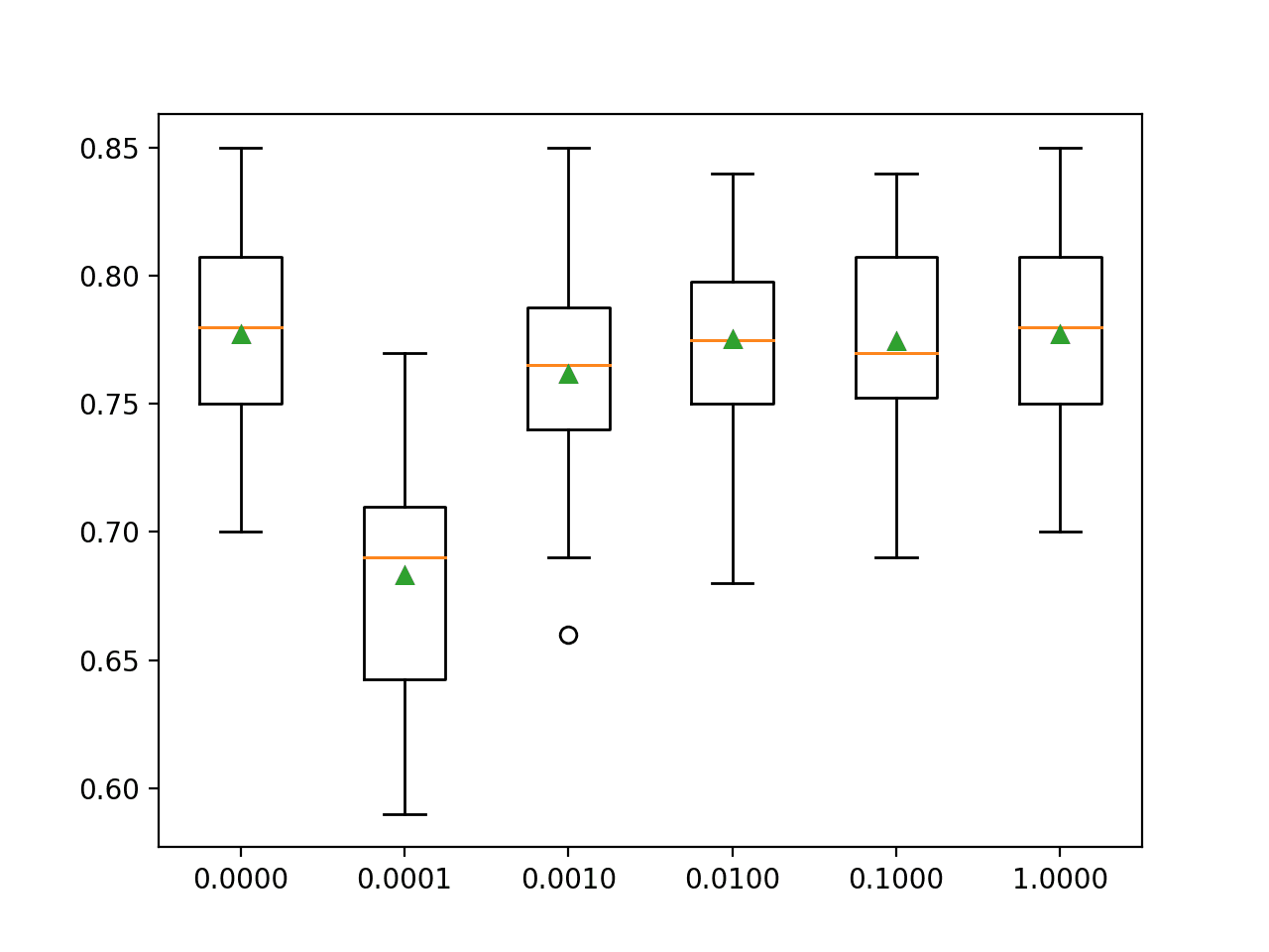
Viewing all 263 articles
Browse latest View live